COMPACT HIGHER-ORDER AMBISONIC LIBRARY
Contents
- ENERGY AND VELOCITY VECTOR ANALYSIS
- SAMPLING DECODING (SAD)
- MODE-MATCHING DECODING (MMD)
- ENERGY-PRESERVING DECODING (EPAD)
- ALL-ROUND AMBISONIC DECODING (ALLRAD)
- CONSTANT ANGULAR SPREAD DECODING (CSAD)
- THE MAX-rE WEIGHTING
- ENCODING/DECODING AMBISONIC SIGNALS
- FREQUENCY DEPENDENT-DECODING
- ROTATION OF AMBISONIC SOUND SCENES (REQUIRES THE SHT-LIB)
- CONVERSION BETWEEN DIFFERENT FORMATS
- REFERENCES
%%%%%%%%%%%%%%%%%%%%%%%%%%%%%%%%%%%%%%%%%%%%%%%%%%%%%%%%%%%%%%%%%%%%%%%%%%%%
%
%   Archontis Politis, 2015
%   Department of Signal Processing and Acoustics, Aalto University, Finland
%   archontis.politis@aalto.fi
%
%%%%%%%%%%%%%%%%%%%%%%%%%%%%%%%%%%%%%%%%%%%%%%%%%%%%%%%%%%%%%%%%%%%%%%%%%%%%
This is a compact Matlab/Octave library implementing most common operations associated with higher-order ambisonics (HOA), which refer to a set of spatial audio techniques for capturing, manipulating and reproducing sound scenes, based on a spherical Fourier expansion of the sound field.
The included functions implement HOA encoding of directional sounds, decoding using various decoding approaches, and rotation of HOA sound scenes. All operations are defined in terms of orthonormalized real Spherical Harmonics (N3D in ambisonic slang) and channel indexing according to  , where n is the order and m is the degree (ACN in ambisonic slang). However, functions are included to convert to and from N3D/ACN to some other established conventions (namely semi-normalized SHs (SN3D) and an alternative channel indexing, termed SID).
Ambisonic decoding can be approached from various sides, more physically inspired or more perceptually inspired. Five approaches are implemented
- 1) Sampling or projection decoding (transpose)
- 2) Mode-matching decoding (pseudo-inverse)
- 3) Energy-preserving decoding [ref.1]
- 4) All-round ambisonic decoding [ref.2]
- 5) Constant-angular spread decoding [ref.3]
Apart from the two first traditional approaches, the three last are more recent and more perceptually motivated. They are also more flexible and robust, in terms of loudspeaker layouts.
Additionally, a function evaluating and visualizing the popular ambisonic performance measures, velocity and energy vectors, along with overall energy and amplitude preservation, is included.
Max-rE weighting for the decoder [ref.4 & ref.2] can be optionally enabled.
ALLRAD and CSAD decoders require computation of amplitude and energy panning gains, and large spherical uniform sampling schemes (t-Designs). Both of these can be found firs in the Matlab/Octave VBAP library in
https://github.com/polarch/Vector-Base-Amplitude-Panning
and the general Spherical harmonic transform library by the author found in
https://github.com/polarch/Spherical-Harmonic-Transform,
These two libraries should be added to the Matlab path before executing this script.
Rotation, apart from the case of simple B-format, also depends on the larger spherical harmonic transform library, which contains many other operations that may be of interest to ambisonics, like directional smoothing (spherical convolution) and directional weighting/shaping (spherical multiplication).
The library contains the following main functions:
- ambiDecoder: Compute a HOA decoding matrix for a specified order and a specified method, with or without max-rE weighting
- analyzeDecoder: Analyze amplitude, energy, velocity and energy vector magnitudes and directional errors and spread, for an ambisonic decoder, or from panning gains
- getRSH: returns values of real orthonormal spherical harmonics vectors of directions
- encodeHOA_N3D: encode a number of source signals from various directions to arbitrary-order HOA signals (N3D, ACN)
- encodeBformat: encode a number of source signals from various directions to traditional B-format signals
- decodeHOA_N3D: decode HOA signals to a loudspeaker setup, using a certain decoding matrix (frequency-dependent decoding possible, see below)
- decodeBformat: decode B-format signals to a loudspeaker setup, using a certain decoding matrix
- rotateHOA_N3D: rotate sound scenes encoded or recorded in HOA signals, using a yaw-pitch-roll convention
- rotateBformat: rotate sound scenes encoded or recorded to B-format signals, using a yaw-pitch-roll convention
- allrad: implements the all-round ambisonic decoder
- csad: implements the constant-angular spread decoder
- getLayoutAmbisonicOrder: Compute the equivalent ambisonic order for regular and irregular speaker arrangements
- getMaxREweights: Compute the max-rE weights for a certain order, for decoding (or encoding) weighting
- getTheoreticalEVmag: Compute the theoretical energy vector magnitude of a plane-wave encoded to a certain order, with max-rE weighting
- plotSphericalGrid: Plots angular quantities in a 2D azimuth-elevation grid, with loudspeaker positions superimposed
For any questions, comments, corrections, or general feedback, please contact archontis.politis@aalto.fi
ENERGY AND VELOCITY VECTOR ANALYSIS
The velocity (or Makita) vector [ref.5] and the energy (or Gerzon) vector [ref.6], computed from the loudspeaker layout and the panning gains for a certain panning direction, are believed to indicate perceived directions along with localization blur and source spread. These two vectors are actually related to the more general acoustic intensity vector, and the diffuseness or reactivity of the soundfield at the listening spot, but they are simpler to compute (see [ref.7]). They have been fundamental in the design of ambisonic systems. Psychoacoustical validation of their relation to localization attributes has only recently been studied [ref.8].
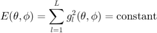
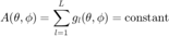
Generally, loudspeaker gains have to preserve the energy of a sound coming from a certain direction, so that the loudspeaker setup does not affect its loudness. This energy preservation property can be given as:
while at low frequencies it is more appropriate to preserve the total amplitude, since a coherent summation model at the listener's ears is more appropriate (see [ref.9])
 .
.
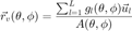
Here  denote azimuth and elevation, and
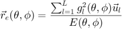
  are the loudspeaker gains for the specific direction. Velocity and energy vectors are then given by
and
 .
.
where  are the unit vectors pointing to the speakers. Analysis of a panner or decoder in terms of energy/amplitude preservation and velocity/energy vectors can be done with analyzeDecoder().
In terms of ambisonic decoding, for a uniform arrangement of loudspeakers, the ambisonic order of the layout can be readily given by
 .
.
For irregular layouts, evaluating an effective order is more complicated, Zotter & Frank in [ref.2] propose an equivalent ambisonic order having to do with the average spread of the layout. The equivalent ambisonic order can be evaluated here by getLayoutAmbisonicOrder().
A relation of the source spread/localization blur, with repect to the magnitude of the energy vector is given by Daniel or Zotter in [ref.4 & 2]
 .
.
while an alternative definition is given by Epain et al. in [ref.3]
 .
.
Finally, Frank in [ref.10] proposes a psychoacoustic curve between the relation of the enegry vector magnitude and perceived spread, from listening tests:
 .
.
In any case, the best energy vector magnitude, and so minimal spread, that can be achieved for a certain decoding order (due to a theoretical continuous ambisonic loudspeaker setup) is given by [ref.4 & 2]
 .
.
where  are the per-order decoding weights, such as the max-rE ones. These metrics for a certain panner/decoder are displayed if the flag INFO_ON on the analyzeDecoder() is set to true.
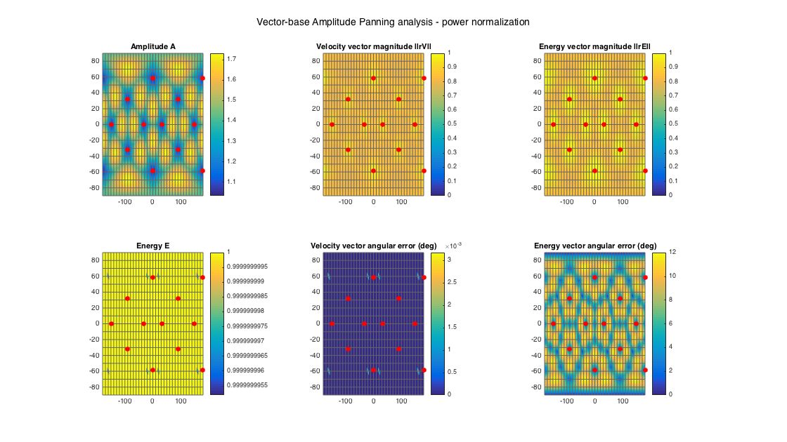
A first example is shown for pure amplitude panning (and energy panning) functions, which are not ambisonic but they serve as basis for some of the more flexible ambisonic decoders included here.
% define a 3D layout with the shape of an icosahedron
[~, ls_dirs_rad] = platonicSolid('icosahedron');
ls_dirs = ls_dirs_rad*180/pi;
ls_num = size(ls_dirs,1);

aziRes = 5;
polarRes = 5;
ang_res = [aziRes polarRes];
g_vbap = getGainTable(ls_dirs, ang_res, 0, 'vbap');
[g_vbip, g_dirs] = getGainTable(ls_dirs, ang_res, 0, 'vbip');

% reshape the 1D array of gains (times ls_num) returned by getGainTable()
% to a 2D azimuth-elevation matrix (times ls_num)
G_vbap = permute(reshape(g_vbap, [(360/aziRes+1) (180/polarRes+1) ls_num]), [2 1 3]);
G_vbip = permute(reshape(g_vbip, [(360/aziRes+1) (180/polarRes+1) ls_num]), [2 1 3]);

% analyze and plot panners for the grid of panning directions on the gain
% table
analyzeDecoder(G_vbap, ls_dirs, 'panner', ang_res, 1, 1);
h = gcf; h.Position(3) = 2*h.Position(3); h.Position(4) = 1.5*h.Position(4);
suptitle('Vector-base Amplitude Panning analysis - power normalization')
Amplitude range: 0.28567 ~ 4.7709 dB
Energy range: -2.0878e-08 ~ 1.9287e-15 dB
Directional error range of rV: 0 ~ 0.0031734 deg
Directional error range of rE: 0 ~ 12.0233 deg
Magnitude range of rV: 0.79466 ~ 0.98225
Magnitude range of rE: 0.79469 ~ 0.99936
Spread range of rE (Daniel): 4.0968 ~ 74.7483 deg
Spread range of rE (Frank): 10.8191 ~ 48.9701 deg
Spread range of rE (Epain et al.): 5.7941 ~ 107.7744 deg
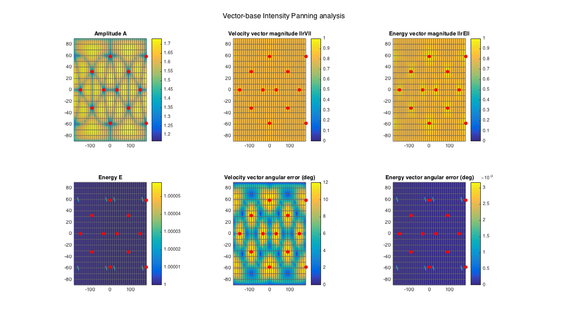
analyzeDecoder(G_vbip, ls_dirs, 'panner', ang_res, 1, 1);
h = gcf; h.Position(3) = 2*h.Position(3); h.Position(4) = 1.5*h.Position(4);
suptitle('Vector-base Intensity Panning analysis')
Amplitude range: 1.3252 ~ 4.7711 dB
Energy range: -1.4465e-15 ~ 0.00025197 dB
Directional error range of rV: 0 ~ 12.0685 deg
Directional error range of rE: 0 ~ 0.0031734 deg
Magnitude range of rV: 0.79466 ~ 0.92446
Magnitude range of rE: 0.79466 ~ 0.98225
Spread range of rE (Daniel): 21.6246 ~ 74.7531 deg
Spread range of rE (Frank): 14.0092 ~ 48.9748 deg
Spread range of rE (Epain et al.): 30.6276 ~ 107.7816 deg
% an example of re-normalized vbap gains for amplitude normalization, e.g.
% suitable for low frequencies
g_vbap_renorm = g_vbap./( sum(g_vbap,2)*ones(1,ls_num) );
G_vbap_renorm = permute(reshape(g_vbap_renorm, [(360/aziRes+1) (180/polarRes+1) ls_num]), [2 1 3]);
analyzeDecoder(G_vbap_renorm, ls_dirs, 'panner', ang_res, 1, 1);
h = gcf; h.Position(3) = 2*h.Position(3); h.Position(4) = 1.5*h.Position(4);
suptitle('Vector-base Amplitude Panning analysis - amplitude normalization')
Amplitude range: -1.9287e-15 ~ 1.9287e-15 dB
Energy range: -4.7709 ~ -0.28567 dB
Directional error range of rV: 0 ~ 0.0031734 deg
Directional error range of rE: 0 ~ 12.0233 deg
Magnitude range of rV: 0.79466 ~ 0.98225
Magnitude range of rE: 0.79469 ~ 0.99936
Spread range of rE (Daniel): 4.0968 ~ 74.7483 deg
Spread range of rE (Frank): 10.8191 ~ 48.9701 deg
Spread range of rE (Epain et al.): 5.7941 ~ 107.7744 deg
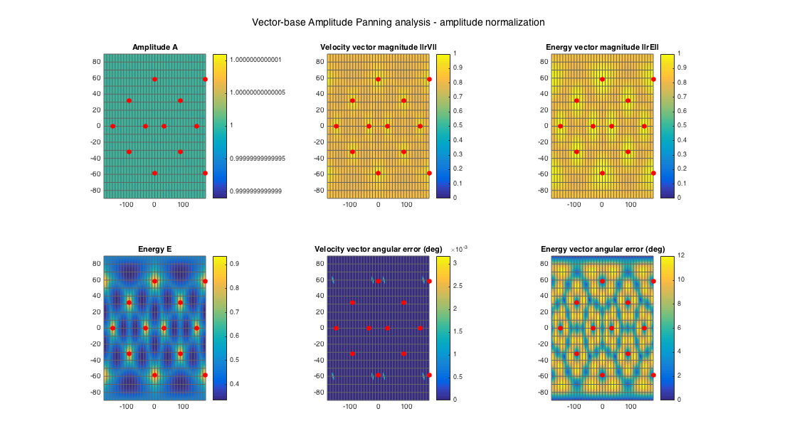
It is evident that VBAP maximises the velocity vector, with zero directional error, while VBIP maximises the energy vector, with zero directional error. Both of them produce very high magnitudes for the two vectors since they use the minimal number of loudspeakers, at the expense of a variable spread with direction (which is otherwie also the minimum possible for each direction).
SAMPLING DECODING (SAD)
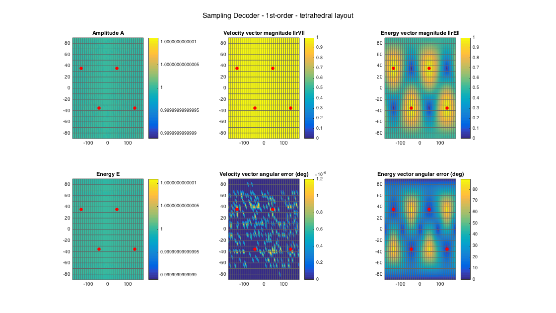
The sampling, or projection, decoder, is the simplest, and essentially corresponds to a plane-wave decomposition at the direction of each loudspeaker, band-limited to the supported order of the layout (an alternative interpretation is that the decoder forms higher-order hypercardioids, or virtual microphones in ambisonic slang, to the direction of the loudspeakers). It is easy to see how this decoder would be robust to irregular loudspeaker layouts, but it won't preserve the energy of a source or localization cues for all directions.
In the following example, analysis plots are generated for a uniform minimal 1st-order layout, a uniform 3rd-order layout, and a 22.0 irregular setup.
% tetrahedral setup
[~, ls_dirs4_rad] = platonicSolid('tetra');
ls_dirs4 = ls_dirs4_rad*180/pi;
ls_num = size(ls_dirs4,1);

% get order (1 in this case)
N = floor(sqrt(ls_num) - 1);
% get a sampling decoder
D_sad4 = ambiDecoder(ls_dirs4, 'sad', 0, N);
% analyze decoder properties
analyzeDecoder(D_sad4, ls_dirs4, 'decoder', [5 5], 1, 1);
h = gcf; h.Position(3) = 2*h.Position(3); h.Position(4) = 1.5*h.Position(4);
suptitle(['Sampling Decoder - ' num2str(N) 'st-order - tetrahedral layout'])
Amplitude range: -3.8573e-15 ~ 1.9287e-15 dB
Energy range: -3.3751e-15 ~ 3.8573e-15 dB
Directional error range of rV: 0 ~ 1.2074e-06 deg
Directional error range of rE: 0 ~ 89.6036 deg
Magnitude range of rV: 1 ~ 1
Magnitude range of rE: 0.004622 ~ 0.99998
Spread range of rE (Daniel): 0.74781 ~ 179.4704 deg
Spread range of rE (Frank): 10.704 ~ 196.2385 deg
Spread range of rE (Epain et al.): 1.0576 ~ 344.4069 deg
Equivalent ambisonic order of layout: 1
Theoretical magnitude of rE for equivalent order: 0.57152
Theoretical magnitude of rE for decoding order: 0.57152
Theoretical spread of equivalent order (Daniel): 110.2877
Theoretical spread of decoding order (Daniel): 110.2877
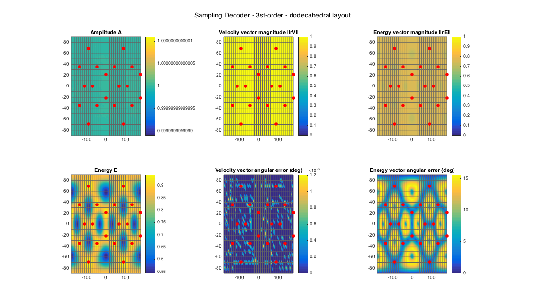
% dodecahedral setup
[~, ls_dirs20_rad] = platonicSolid('dodecahedron');
ls_dirs20 = ls_dirs20_rad*180/pi;
ls_num = size(ls_dirs20,1);
% get order (3 in this case)
N = floor(sqrt(ls_num) - 1);
% get a projection (sampling) decoder
D_sad20 = ambiDecoder(ls_dirs20, 'sad', 0, N);
% analyze decoder properties
analyzeDecoder(D_sad20, ls_dirs20, 'decoder', [5 5], 1, 1);
h = gcf; h.Position(3) = 2*h.Position(3); h.Position(4) = 1.5*h.Position(4);
suptitle(['Sampling Decoder - ' num2str(N) 'st-order - dodecahedral layout'])
Amplitude range: -8.6789e-15 ~ 9.6433e-15 dB
Energy range: -2.6506 ~ -0.25028 dB
Directional error range of rV: 0 ~ 1.2074e-06 deg
Directional error range of rE: 0 ~ 15.5844 deg
Magnitude range of rV: 1 ~ 1
Magnitude range of rE: 0.70065 ~ 0.76865
Spread range of rE (Daniel): 79.5338 ~ 91.0423 deg
Spread range of rE (Frank): 53.8231 ~ 66.4996 deg
Spread range of rE (Epain et al.): 114.9992 ~ 132.6821 deg
Equivalent ambisonic order of layout: 3
Theoretical magnitude of rE for equivalent order: 0.86077
Theoretical magnitude of rE for decoding order: 0.86077
Theoretical spread of equivalent order (Daniel): 61.1947
Theoretical spread of decoding order (Daniel): 61.1947
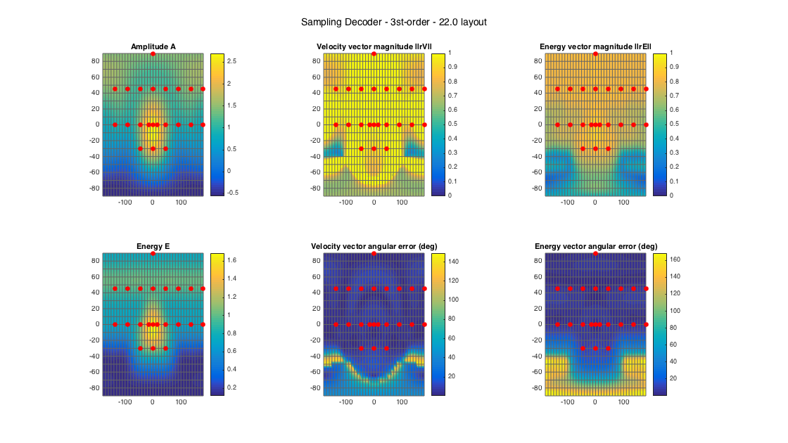
% 22.2 style loudspeaker layout - quite irregular
ls_dirs22 = [45 -45 0 135 -135 15 -15 90 -90 180 45 -45  0 135 -135 90 -90 180  0  45 -45   0;
              0   0 0   0    0  0   0  0   0   0 45  45 45  45   45 45  45  45 90 -30 -30 -30]';
ls_num = size(ls_dirs22,1);
% get order
N = floor(sqrt(ls_num) - 1);
% get ambisonic equivalent order, for comparison
Neq = getLayoutAmbisonicOrder(ls_dirs);
% get a projection (sampling) decoder
D_sad22 = ambiDecoder(ls_dirs22, 'sad', 0, N);
% analyze decoder properties
analyzeDecoder(D_sad22, ls_dirs22, 'decoder', [5 5], 1, 1);
h = gcf; h.Position(3) = 2*h.Position(3); h.Position(4) = 1.5*h.Position(4);
suptitle(['Sampling Decoder - ' num2str(N) 'st-order - 22.0 layout'])
Amplitude range: -5.05702+27.2875i ~ 8.6272 dB
Energy range: -9.3925 ~ 2.2763 dB
Directional error range of rV: 0.21333 ~ 149.2134 deg
Directional error range of rE: 0.037013 ~ 168.5191 deg
Magnitude range of rV: 0.2452 ~ 68.4539
Magnitude range of rE: 0.11728 ~ 0.88448
Spread range of rE (Daniel): 55.6244 ~ 166.5299 deg
Spread range of rE (Frank): 32.2326 ~ 175.2393 deg
Spread range of rE (Epain et al.): 79.4782 ~ 279.8928 deg
Equivalent ambisonic order of layout: 3
Theoretical magnitude of rE for equivalent order: 0.86077
Theoretical magnitude of rE for decoding order: 0.86077
Theoretical spread of equivalent order (Daniel): 61.1947
Theoretical spread of decoding order (Daniel): 61.1947
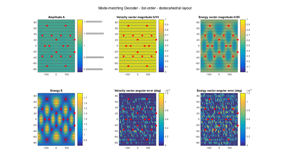
MODE-MATCHING DECODING (MMD)
The mode-matching decoder is the most 'physically'-based decoder, and it results from equating the spherical expansion of a plane wave for an arbitrary direction, to a weighted spherical expansion of the plane waves emitted by the loudspeaker setup, solving for the weights in a least-square sense. The solution is simply the pseudo-inverse of the SHs on the direction of the speakers. Even though, mode-matching is an exact solution at some small region (order and frequency-dependent) around the sweet-spot, in practice it is useful only at low frequencies, and only for regular layouts, as it is very sensitive to irregularities.
In the following example, analysis plots are generated for a uniform minimal 1st-order layout, a uniform 3rd-order layout, and a 22.0 irregular setup.
% tetrahedral setup
[~, ls_dirs4_rad] = platonicSolid('tetra');
ls_dirs4 = ls_dirs4_rad*180/pi;
ls_num = size(ls_dirs4,1);

% get order (1 in this case)
N = floor(sqrt(ls_num) - 1);
% get a MMD
D_mmd4 = ambiDecoder(ls_dirs4, 'mmd', 0, N);
% analyze decoder properties
analyzeDecoder(D_mmd4, ls_dirs4, 'decoder', [5 5], 1, 1);
h = gcf; h.Position(3) = 2*h.Position(3); h.Position(4) = 1.5*h.Position(4);
suptitle(['Mode-matching Decoder - ' num2str(N) 'st-order - tetrahedral layout'])
Amplitude range: -9.6433e-15 ~ 3.8573e-15 dB
Energy range: -5.3038e-15 ~ 3.8573e-15 dB
Directional error range of rV: 0 ~ 1.2074e-06 deg
Directional error range of rE: 0 ~ 89.6036 deg
Magnitude range of rV: 1 ~ 1
Magnitude range of rE: 0.004622 ~ 0.99998
Spread range of rE (Daniel): 0.74781 ~ 179.4704 deg
Spread range of rE (Frank): 10.704 ~ 196.2385 deg
Spread range of rE (Epain et al.): 1.0576 ~ 344.4069 deg
Equivalent ambisonic order of layout: 1
Theoretical magnitude of rE for equivalent order: 0.57152
Theoretical magnitude of rE for decoding order: 0.57152
Theoretical spread of equivalent order (Daniel): 110.2877
Theoretical spread of decoding order (Daniel): 110.2877

% dodecahedral setup
[~, ls_dirs20_rad] = platonicSolid('dodecahedron');
ls_dirs20 = ls_dirs20_rad*180/pi;
ls_num = size(ls_dirs20,1);
% get order (3 in this case)
N = floor(sqrt(ls_num) - 1);
% get a MMD
D_mmd20 = ambiDecoder(ls_dirs20, 'mmd', 0, N);
% analyze decoder properties
analyzeDecoder(D_mmd20, ls_dirs20, 'decoder', [5 5], 1, 1);
h = gcf; h.Position(3) = 2*h.Position(3); h.Position(4) = 1.5*h.Position(4);
suptitle(['Mode-matching Decoder - ' num2str(N) 'st-order - dodecahedral layout'])
Amplitude range: -1.5429e-14 ~ 1.1572e-14 dB
Energy range: -0.96867 ~ 2.5381 dB
Directional error range of rV: 0 ~ 1.2074e-06 deg
Directional error range of rE: 0 ~ 1.2074e-06 deg
Magnitude range of rV: 1 ~ 1
Magnitude range of rE: 0.33446 ~ 0.74992
Spread range of rE (Daniel): 82.8322 ~ 140.9209 deg
Spread range of rE (Frank): 57.314 ~ 134.7571 deg
Spread range of rE (Epain et al.): 120.0199 ~ 218.6692 deg
Equivalent ambisonic order of layout: 3
Theoretical magnitude of rE for equivalent order: 0.86077
Theoretical magnitude of rE for decoding order: 0.86077
Theoretical spread of equivalent order (Daniel): 61.1947
Theoretical spread of decoding order (Daniel): 61.1947
% 22.2 style loudspeaker layout - quite irregular
ls_dirs22 = [45 -45 0 135 -135 15 -15 90 -90 180 45 -45  0 135 -135 90 -90 180  0  45 -45   0;
              0   0 0   0    0  0   0  0   0   0 45  45 45  45   45 45  45  45 90 -30 -30 -30]';
ls_num = size(ls_dirs22,1);
% get order
N = floor(sqrt(ls_num) - 1);
% get a MMD
D_mmd22 = ambiDecoder(ls_dirs22, 'mmd', 0, N);
% analyze decoder properties
analyzeDecoder(D_mmd22, ls_dirs22, 'decoder', [5 5], 1, 1);
h = gcf; h.Position(3) = 2*h.Position(3); h.Position(4) = 1.5*h.Position(4);
suptitle(['Mode-matching Decoder - ' num2str(N) 'st-order - 22.0 layout'])
Amplitude range: -6.9432e-14 ~ 3.2787e-14 dB
Energy range: -4.4987 ~ 25.5989 dB
Directional error range of rV: 0 ~ 1.2074e-06 deg
Directional error range of rE: 0 ~ 175.8335 deg
Magnitude range of rV: 1 ~ 1
Magnitude range of rE: 0.16088 ~ 1
Spread range of rE (Daniel): 0 ~ 161.4836 deg
Spread range of rE (Frank): 10.7 ~ 167.1113 deg
Spread range of rE (Epain et al.): 0 ~ 265.4114 deg
Equivalent ambisonic order of layout: 3
Theoretical magnitude of rE for equivalent order: 0.86077
Theoretical magnitude of rE for decoding order: 0.86077
Theoretical spread of equivalent order (Daniel): 61.1947
Theoretical spread of decoding order (Daniel): 61.1947
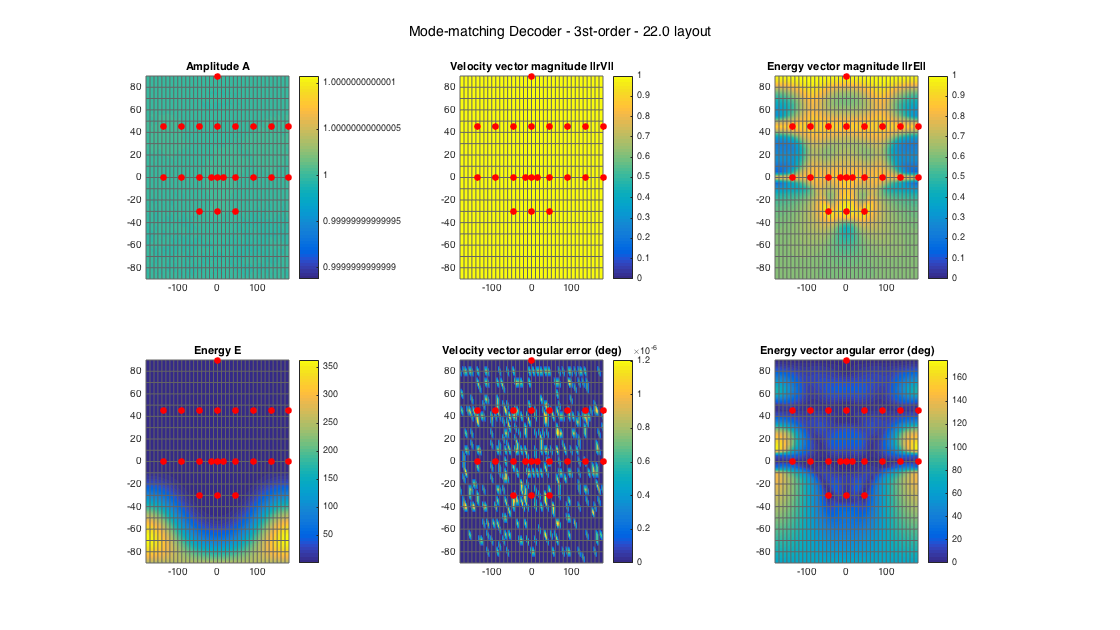
Mode-matching is problematic for irregular layouts, due to the inversion of the sampling matrix that becomes unstable - the effect can be seen at the energy amplification at directions for which the layout is quite sparse.
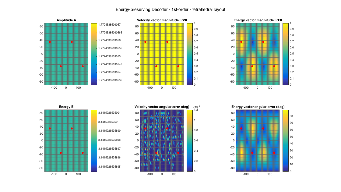
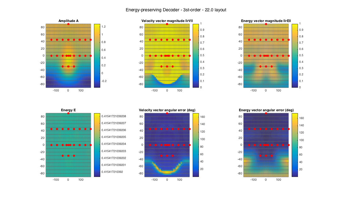
ENERGY-PRESERVING DECODING (EPAD)
This approach has been devised by Zotter et al [ref.1] to address the energy-preserving issues of the previous two basic decoding approaches, especially for irregular layouts. It resembles the projection decoding, but with an additional singular value decomposition of the sampling matrix, appropriate truncation and omission of the singular values, resulting in a semi-orthogonal decoding matrix that preserves energy.
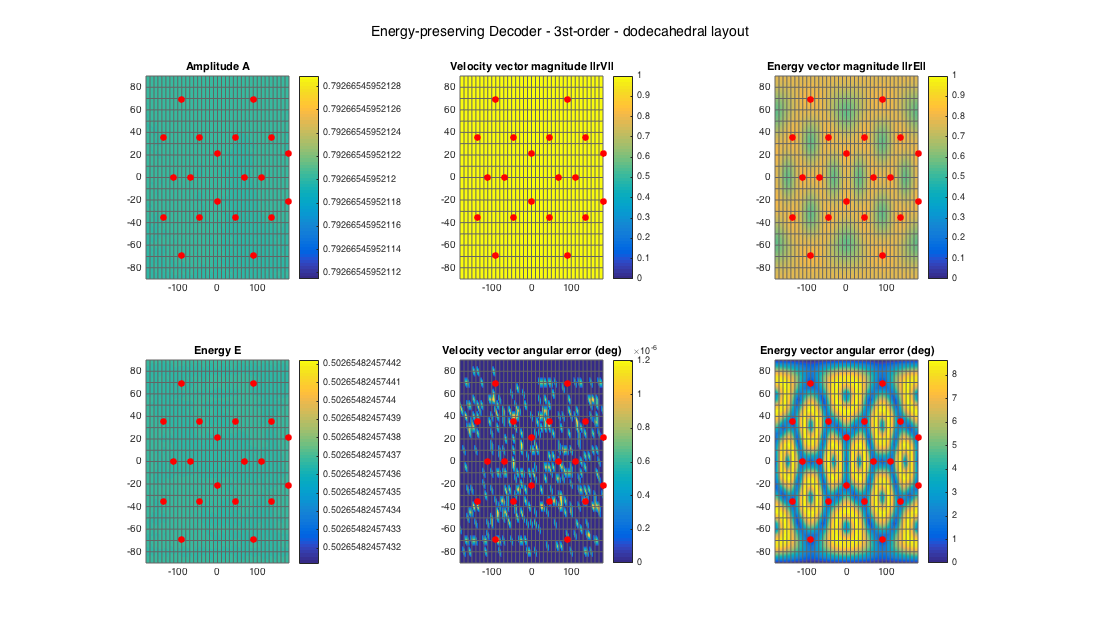
In the following example, analysis plots are generated for a uniform minimal 1st-order layout, a uniform 3rd-order layout, and a 22.0 irregular setup.
% tetrahedral setup
[~, ls_dirs4_rad] = platonicSolid('tetra');
ls_dirs4 = ls_dirs4_rad*180/pi;
ls_num = size(ls_dirs4,1);

% get order (1 in this case)
N = floor(sqrt(ls_num) - 1);
% get an EPAD
D_epad4 = ambiDecoder(ls_dirs4, 'epad', 0, N);
% analyze decoder properties
analyzeDecoder(D_epad4, ls_dirs4, 'decoder', [5 5], 1, 1);
h = gcf; h.Position(3) = 2*h.Position(3); h.Position(4) = 1.5*h.Position(4);
suptitle(['Energy-preserving Decoder - ' num2str(N) 'st-order - tetrahedral layout'])
Amplitude range: 4.9715 ~ 4.9715 dB
Energy range: 4.9715 ~ 4.9715 dB
Directional error range of rV: 0 ~ 1.2074e-06 deg
Directional error range of rE: 0 ~ 89.6036 deg
Magnitude range of rV: 1 ~ 1
Magnitude range of rE: 0.004622 ~ 0.99998
Spread range of rE (Daniel): 0.74781 ~ 179.4704 deg
Spread range of rE (Frank): 10.704 ~ 196.2385 deg
Spread range of rE (Epain et al.): 1.0576 ~ 344.4069 deg
Equivalent ambisonic order of layout: 1
Theoretical magnitude of rE for equivalent order: 0.57152
Theoretical magnitude of rE for decoding order: 0.57152
Theoretical spread of equivalent order (Daniel): 110.2877
Theoretical spread of decoding order (Daniel): 110.2877
% dodecahedral setup
[~, ls_dirs20_rad] = platonicSolid('dodecahedron');
ls_dirs20 = ls_dirs20_rad*180/pi;
ls_num = size(ls_dirs20,1);
% get order (3 in this case)
N = floor(sqrt(ls_num) - 1);
% get an EPAD
D_epad20 = ambiDecoder(ls_dirs20, 'epad', 0, N);
% analyze decoder properties
analyzeDecoder(D_epad20, ls_dirs20, 'decoder', [5 5], 1, 1);
h = gcf; h.Position(3) = 2*h.Position(3); h.Position(4) = 1.5*h.Position(4);
suptitle(['Energy-preserving Decoder - ' num2str(N) 'st-order - dodecahedral layout'])
Amplitude range: -2.0182 ~ -2.0182 dB
Energy range: -2.9873 ~ -2.9873 dB
Directional error range of rV: 0 ~ 1.2074e-06 deg
Directional error range of rE: 0 ~ 8.6434 deg
Magnitude range of rV: 1 ~ 1
Magnitude range of rE: 0.56767 ~ 0.81194
Spread range of rE (Daniel): 71.4288 ~ 110.8242 deg
Spread range of rE (Frank): 45.755 ~ 91.2864 deg
Spread range of rE (Epain et al.): 102.8009 ~ 164.4435 deg
Equivalent ambisonic order of layout: 3
Theoretical magnitude of rE for equivalent order: 0.86077
Theoretical magnitude of rE for decoding order: 0.86077
Theoretical spread of equivalent order (Daniel): 61.1947
Theoretical spread of decoding order (Daniel): 61.1947
% 22.2 style loudspeaker layout - quite irregular
ls_dirs22 = [45 -45 0 135 -135 15 -15 90 -90 180 45 -45  0 135 -135 90 -90 180  0  45 -45   0;
              0   0 0   0    0  0   0  0   0   0 45  45 45  45   45 45  45  45 90 -30 -30 -30]';
ls_num = size(ls_dirs22,1);
% get order
N = floor(sqrt(ls_num) - 1);
% get an EPAD
D_epad22 = ambiDecoder(ls_dirs22, 'epad', 0, N);
% analyze decoder properties
analyzeDecoder(D_epad22, ls_dirs22, 'decoder', [5 5], 1, 1);
h = gcf; h.Position(3) = 2*h.Position(3); h.Position(4) = 1.5*h.Position(4);
suptitle(['Energy-preserving Decoder - ' num2str(N) 'st-order - 22.0 layout'])
Amplitude range: -8.72583+27.2875i ~ 2.1494 dB
Energy range: -3.8152 ~ -3.8152 dB
Directional error range of rV: 0.010137 ~ 170.5023 deg
Directional error range of rE: 0.030186 ~ 174.5717 deg
Magnitude range of rV: 0.065859 ~ 37.663
Magnitude range of rE: 0.27091 ~ 0.91281
Spread range of rE (Daniel): 48.2069 ~ 148.5626 deg
Spread range of rE (Frank): 26.9523 ~ 146.6016 deg
Spread range of rE (Epain et al.): 68.6974 ~ 234.5383 deg
Equivalent ambisonic order of layout: 3
Theoretical magnitude of rE for equivalent order: 0.86077
Theoretical magnitude of rE for decoding order: 0.86077
Theoretical spread of equivalent order (Daniel): 61.1947
Theoretical spread of decoding order (Daniel): 61.1947
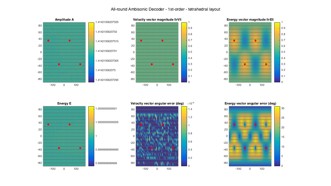
ALL-ROUND AMBISONIC DECODING (ALLRAD)
ALLRAD is one of the two more advanced and flexible decoding approaches, implemented here. It has been presented by Zotter anf Frank in [ref.2] and manages to handle well irregular loudspeaker setups, with low directional error and with good energy-preserving properties. This is achieved by a combination of amplitude panning (VBAP) stage rendering virtual sources that correspond to a uniform dense arrangement, which due to its uniformity satisfies all ambisonic analysis requirements. The VBAP renders this virtual ideal decoder to an arbitrary layout.
In the following example, analysis plots are generated for a uniform minimal 1st-order layout, a uniform 3rd-order layout, and a 22.0 irregular setup.
% tetrahedral setup
[~, ls_dirs4_rad] = platonicSolid('tetra');
ls_dirs4 = ls_dirs4_rad*180/pi;
ls_num = size(ls_dirs4,1);

% get order (1 in this case)
N = floor(sqrt(ls_num) - 1);
% get an ALLRAD
D_allrad4 = ambiDecoder(ls_dirs4, 'allrad', 0, N);
% analyze decoder properties
analyzeDecoder(D_allrad4, ls_dirs4, 'decoder', [5 5], 1, 1);
h = gcf; h.Position(3) = 2*h.Position(3); h.Position(4) = 1.5*h.Position(4);
suptitle(['All-round Ambisonic Decoder - ' num2str(N) 'st-order - tetrahedral layout'])
Amplitude range: 3.0103 ~ 3.0103 dB
Energy range: -2.893e-15 ~ 4.8216e-15 dB
Directional error range of rV: 0 ~ 1.4788e-06 deg
Directional error range of rE: 0 ~ 31.2223 deg
Magnitude range of rV: 0.57735 ~ 0.57735
Magnitude range of rE: 0.24406 ~ 0.91067
Spread range of rE (Daniel): 48.8045 ~ 151.7477 deg
Spread range of rE (Frank): 27.3516 ~ 151.6076 deg
Spread range of rE (Epain et al.): 69.5627 ~ 241.5789 deg
Equivalent ambisonic order of layout: 1
Theoretical magnitude of rE for equivalent order: 0.57152
Theoretical magnitude of rE for decoding order: 0.57152
Theoretical spread of equivalent order (Daniel): 110.2877
Theoretical spread of decoding order (Daniel): 110.2877
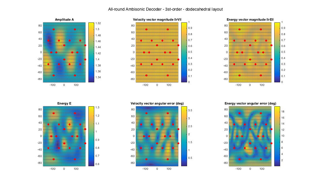
% dodecahedral setup
[~, ls_dirs20_rad] = platonicSolid('dodecahedron');
ls_dirs20 = ls_dirs20_rad*180/pi;
ls_num = size(ls_dirs20,1);
% get order (3 in this case)
N = floor(sqrt(ls_num) - 1);
% get an ALLRAD
D_allrad20 = ambiDecoder(ls_dirs20, 'allrad', 0, N);
% analyze decoder properties
analyzeDecoder(D_allrad20, ls_dirs20, 'decoder', [5 5], 1, 1);
h = gcf; h.Position(3) = 2*h.Position(3); h.Position(4) = 1.5*h.Position(4);
suptitle(['All-round Ambisonic Decoder - ' num2str(N) 'st-order - dodecahedral layout'])
Amplitude range: 2.4426 ~ 3.658 dB
Energy range: -2.3845 ~ 1.2024 dB
Directional error range of rV: 0.0083 ~ 3.7726 deg
Directional error range of rE: 0.11355 ~ 19.848 deg
Magnitude range of rV: 0.84475 ~ 0.89208
Magnitude range of rE: 0.68473 ~ 0.95645
Spread range of rE (Daniel): 33.9424 ~ 93.5719 deg
Spread range of rE (Frank): 18.8174 ~ 69.4671 deg
Spread range of rE (Epain et al.): 48.1806 ~ 136.6364 deg
Equivalent ambisonic order of layout: 3
Theoretical magnitude of rE for equivalent order: 0.86077
Theoretical magnitude of rE for decoding order: 0.86077
Theoretical spread of equivalent order (Daniel): 61.1947
Theoretical spread of decoding order (Daniel): 61.1947
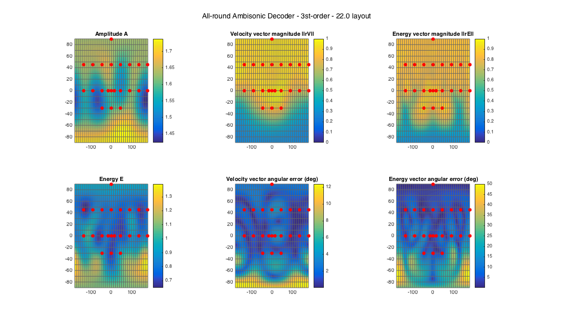
% 22.2 style loudspeaker layout - quite irregular
ls_dirs22 = [45 -45 0 135 -135 15 -15 90 -90 180 45 -45  0 135 -135 90 -90 180  0  45 -45   0;
              0   0 0   0    0  0   0  0   0   0 45  45 45  45   45 45  45  45 90 -30 -30 -30]';
ls_num = size(ls_dirs22,1);
% get order
N = floor(sqrt(ls_num) - 1);
% get an ALLRAD
D_allrad22 = ambiDecoder(ls_dirs22, 'allrad', 0, N);
% analyze decoder properties
analyzeDecoder(D_allrad22, ls_dirs22, 'decoder', [5 5], 1, 1);
h = gcf; h.Position(3) = 2*h.Position(3); h.Position(4) = 1.5*h.Position(4);
suptitle(['All-round Ambisonic Decoder - ' num2str(N) 'st-order - 22.0 layout'])
Amplitude range: 3.0704 ~ 4.8009 dB
Energy range: -1.8716 ~ 1.4359 dB
Directional error range of rV: 0.043804 ~ 12.3844 deg
Directional error range of rE: 0.072957 ~ 50.0526 deg
Magnitude range of rV: 0.25757 ~ 0.99156
Magnitude range of rE: 0.27593 ~ 0.91337
Spread range of rE (Daniel): 48.0483 ~ 147.9647 deg
Spread range of rE (Frank): 26.8471 ~ 145.666 deg
Spread range of rE (Epain et al.): 68.4677 ~ 233.2479 deg
Equivalent ambisonic order of layout: 3
Theoretical magnitude of rE for equivalent order: 0.86077
Theoretical magnitude of rE for decoding order: 0.86077
Theoretical spread of equivalent order (Daniel): 61.1947
Theoretical spread of decoding order (Daniel): 61.1947
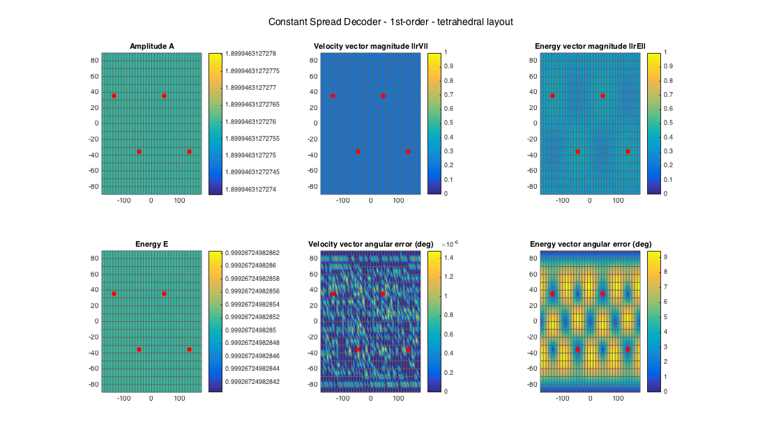
CONSTANT ANGULAR SPREAD DECODING (CSAD)
CSAD is the most recent proposal for flexible and robust ambisonic decoding, proposed by Epain et al. in [ref.3]. Similar to ALLRAD it uses a panning stage, based on VBIP, an energy-based variant of VBAP, in order to derive gains that have zero energy-vector directional error, and additionally they exhibit a constant energy-vector magnitude, which presumable results in a perceptual angular spread/blur that does not change with direction. The resulting VBIP gains are approximated by an ambisonic decoding matrix in a least-squares sense.
The version implemented here is a "lazy-man's" version, since it does not consider the more elaborate smooth windowing of the panning sources in the reference. Instead a plain rectangular angular window is used. However, it seems to perform well, with only small deviations compared to the published results.
In the following example, analysis plots are generated for a uniform minimal 1st-order layout, a uniform 3rd-order layout, and a 22.0 irregular setup.
% tetrahedral setup
[~, ls_dirs4_rad] = platonicSolid('tetra');
ls_dirs4 = ls_dirs4_rad*180/pi;
ls_num = size(ls_dirs4,1);

% get order (1 in this case)
N = floor(sqrt(ls_num) - 1);
% get a CSAD
D_csad4 = ambiDecoder(ls_dirs4, 'csad', 0, N);
% analyze decoder properties
analyzeDecoder(D_csad4, ls_dirs4, 'decoder', [5 5], 1, 1);
h = gcf; h.Position(3) = 2*h.Position(3); h.Position(4) = 1.5*h.Position(4);
suptitle(['Constant Spread Decoder - ' num2str(N) 'st-order - tetrahedral layout'])
Amplitude range: 5.5748 ~ 5.5748 dB
Energy range: -0.0031835 ~ -0.0031835 dB
Directional error range of rV: 0 ~ 1.4788e-06 deg
Directional error range of rE: 0 ~ 9.4598 deg
Magnitude range of rV: 0.18911 ~ 0.18911
Magnitude range of rE: 0.27698 ~ 0.40616
Spread range of rE (Daniel): 132.0726 ~ 147.8399 deg
Spread range of rE (Frank): 121.3922 ~ 145.4709 deg
Spread range of rE (Epain et al.): 201.6354 ~ 232.9797 deg
Equivalent ambisonic order of layout: 1
Theoretical magnitude of rE for equivalent order: 0.57152
Theoretical magnitude of rE for decoding order: 0.57152
Theoretical spread of equivalent order (Daniel): 110.2877
Theoretical spread of decoding order (Daniel): 110.2877
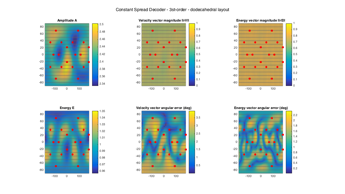
% dodecahedral setup
[~, ls_dirs20_rad] = platonicSolid('dodecahedron');
ls_dirs20 = ls_dirs20_rad*180/pi;
ls_num = size(ls_dirs20,1);
% get order (3 in this case)
N = floor(sqrt(ls_num) - 1);
% get a CSAD
D_csad20 = ambiDecoder(ls_dirs20, 'csad', 0, N);
% analyze decoder properties
analyzeDecoder(D_csad20, ls_dirs20, 'decoder', [5 5], 1, 1);
h = gcf; h.Position(3) = 2*h.Position(3); h.Position(4) = 1.5*h.Position(4);
suptitle(['Constant Spread Decoder - ' num2str(N) 'st-order - dodecahedral layout'])
Amplitude range: 7.3668 ~ 7.9697 dB
Energy range: -0.19121 ~ 0.21498 dB
Directional error range of rV: 0.016525 ~ 3.9449 deg
Directional error range of rE: 0.024022 ~ 2.3703 deg
Magnitude range of rV: 0.65235 ~ 0.75348
Magnitude range of rE: 0.77517 ~ 0.82684
Spread range of rE (Daniel): 68.4485 ~ 78.3589 deg
Spread range of rE (Frank): 42.9765 ~ 52.6081 deg
Spread range of rE (Epain et al.): 98.3599 ~ 113.219 deg
Equivalent ambisonic order of layout: 3
Theoretical magnitude of rE for equivalent order: 0.86077
Theoretical magnitude of rE for decoding order: 0.86077
Theoretical spread of equivalent order (Daniel): 61.1947
Theoretical spread of decoding order (Daniel): 61.1947
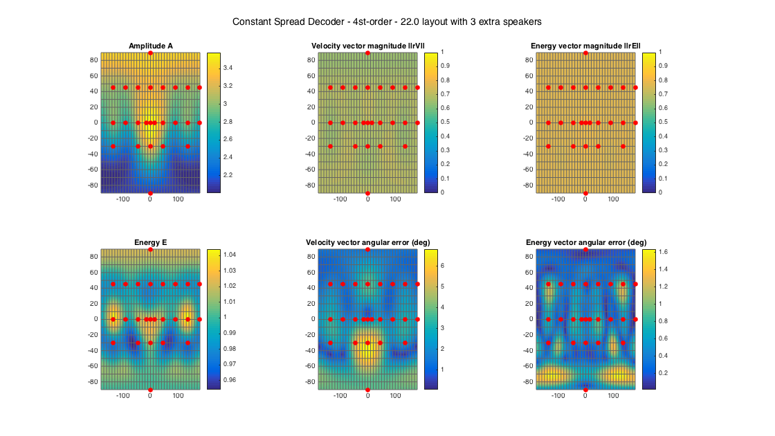
Even though this decoder should be able to handle irregular setups, it seems that (at least the current implementation) the optimization part has difficulties with quite irregular setups like the 22.0 one. In this case, the decoding takes ages to return results and the results themselves are very poor, indicating probably that the optimization fails to converge. (REALLY SLOW!)
% % 22.2 style loudspeaker layout - quite irregular
% ls_dirs22 = [45 -45 0 135 -135 15 -15 90 -90 180 45 -45  0 135 -135 90 -90 180  0  45 -45   0;
%               0   0 0   0    0  0   0  0   0   0 45  45 45  45   45 45  45  45 90 -30 -30 -30]';
% ls_num = size(ls_dirs22,1);
% % get order
% N = floor(sqrt(ls_num) - 1);
% % get a CSAD
% D_csad22 = ambiDecoder(ls_dirs22, 'csad', 0, N);
% % analyze decoder properties
% analyzeDecoder(D_csad22, ls_dirs22, 'decoder', [5 5], 1, 1);
However, giving a more complete irregular setup, based on the 22.0 with only 3 additional speakers, returns fast results with excellent properties.
% 22.2 style loudspeaker layout with 3 extra speakers - more regular
ls_dirs25 = [45 -45 0 135 -135 15 -15 90 -90 180 45 -45  0 135 -135 90 -90 180  0  45 -45   0 135 -135   0;
              0   0 0   0    0  0   0  0   0   0 45  45 45  45   45 45  45  45 90 -30 -30 -30 -30  -30 -90]';
ls_num = size(ls_dirs25,1);
% get order
N = floor(sqrt(ls_num) - 1);
% get a CSAD
D25 = ambiDecoder(ls_dirs25, 'csad', 0, N);
% analyze decoder properties
analyzeDecoder(D25, ls_dirs25, 'decoder', [5 5], 1, 1);
h = gcf; h.Position(3) = 2*h.Position(3); h.Position(4) = 1.5*h.Position(4);
suptitle(['Constant Spread Decoder - ' num2str(N) 'st-order - 22.0 layout with 3 extra speakers'])
Amplitude range: 6.0464 ~ 11.0767 dB
Energy range: -0.2039 ~ 0.18725 dB
Directional error range of rV: 0.053592 ~ 6.8345 deg
Directional error range of rE: 0.012737 ~ 1.6378 deg
Magnitude range of rV: 0.64049 ~ 0.72473
Magnitude range of rE: 0.75928 ~ 0.78578
Spread range of rE (Daniel): 76.4134 ~ 81.1988 deg
Spread range of rE (Frank): 50.6298 ~ 55.5705 deg
Spread range of rE (Epain et al.): 110.2806 ~ 117.529 deg
Equivalent ambisonic order of layout: 4
Theoretical magnitude of rE for equivalent order: 0.90603
Theoretical magnitude of rE for decoding order: 0.90603
Theoretical spread of equivalent order (Daniel): 50.0742
Theoretical spread of decoding order (Daniel): 50.0742
THE MAX-rE WEIGHTING
In ambisonic literature, it is generally believed that the properties of the energy vector are the most crucial for accurate rendering, with the magnitude of the vector related to localization blur, as it was mentioned above. Decoding at mid-high frequencies aims at optimizing the energy vector. Max-rE weighting (actually meaning "max energy vector magnitude" weighting) was introduced by Gerzon for first-order decoders, and formalized by Daniel [ref.4] for higher-order decoders. A derivation is also given by Zotter in [ref.2]. It corresponds to a per-order weighting of the decoder, that results in maximum-norm energy vectors, compared to the unweighted cases like all the previous examples. If a single decoder is used for all frequencies, then max-rE weighting should be preferred, if two (or more) decoding matrices are used for different ranges, then the lowest range should use unweighted decoding (which has maximum velocity vector, suitable for low frequencies) and weighted max-rE at all ranges above. Max-rE can be enabled as a flag in ambiDecoder().
Note the the Constant-angular Spread Decoder (CSAD) maximizes the energy vector (with constraints) by design, so max-rE weighting should not be applied in this case as it will affect its performance.
The example below showcases the unweighted vs. max-rE magnitude of the energy vector, for all of the above decoders and the uniform 20-speaker layout.
ls_num = size(ls_dirs20,1);
% get order (3 in this case)
N = floor(sqrt(ls_num) - 1);
% get max-rE weights up to N
a_n = getMaxREweights(N);
% apply weighting to decoders
D_sad20_maxrE = D_sad20*diag(a_n);
D_mmd20_maxrE = D_mmd20*diag(a_n);
D_epad20_maxrE = D_epad20*diag(a_n);
D_allrad20_maxrE = D_allrad20*diag(a_n);

% Plots
figure
subplot(241)
[~, ~, ~, rE_mag1] = analyzeDecoder(D_sad20, ls_dirs20, 'decoder', ang_res);
plotSphericalGrid(rE_mag1, ang_res, ls_dirs20, gca);
title('SAD - unweighted')
subplot(245)
[~, ~, ~, rE_mag2] = analyzeDecoder(D_sad20_maxrE, ls_dirs20, 'decoder', ang_res);
plotSphericalGrid(rE_mag2, ang_res, ls_dirs20, gca);
title('SAD - max-rE weighting')
subplot(242)
[~, ~, ~, rE_mag1] = analyzeDecoder(D_mmd20, ls_dirs20, 'decoder', ang_res);
plotSphericalGrid(rE_mag1, ang_res, ls_dirs20, gca);
title('MMD - unweighted')
subplot(246)
[~, ~, ~, rE_mag2] = analyzeDecoder(D_mmd20_maxrE, ls_dirs20, 'decoder', ang_res);
plotSphericalGrid(rE_mag2, ang_res, ls_dirs20, gca);
title('MMD - max-rE weighting')
subplot(243)
[~, ~, ~, rE_mag1] = analyzeDecoder(D_epad20, ls_dirs20, 'decoder', ang_res);
plotSphericalGrid(rE_mag1, ang_res, ls_dirs20, gca);
title('EPAD - unweighted')
subplot(247)
[~, ~, ~, rE_mag2] = analyzeDecoder(D_epad20_maxrE, ls_dirs20, 'decoder', ang_res);
plotSphericalGrid(rE_mag2, ang_res, ls_dirs20, gca);
title('EPAD - max-rE weighting')
subplot(244)
[~, ~, ~, rE_mag1] = analyzeDecoder(D_allrad20, ls_dirs20, 'decoder', ang_res);
plotSphericalGrid(rE_mag1, ang_res, ls_dirs20, gca);
title('ALLRAD - unweighted')
subplot(248)
[~, ~, ~, rE_mag2] = analyzeDecoder(D_allrad20_maxrE, ls_dirs20, 'decoder', ang_res, 0);
plotSphericalGrid(rE_mag2, ang_res, ls_dirs20, gca);
title('ALLRAD - max-rE weighting')
h = gcf; h.Position(3) = 2.5*h.Position(3); h.Position(4) = 1.3*h.Position(4);
suptitle('Energy vector magnitude for unweighted and max-rE weighted decoders - dodecahedral layout')
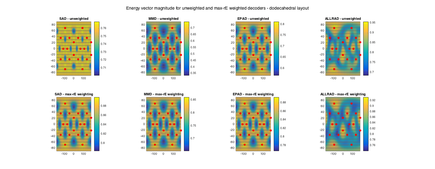
The effect of the max-rE weighting is very pronounced in the case of the 'traditional' decoders, the sampling and mode-matching, while it is smaller in the case of the energy-preserving and all-round decoders.
ENCODING/DECODING AMBISONIC SIGNALS
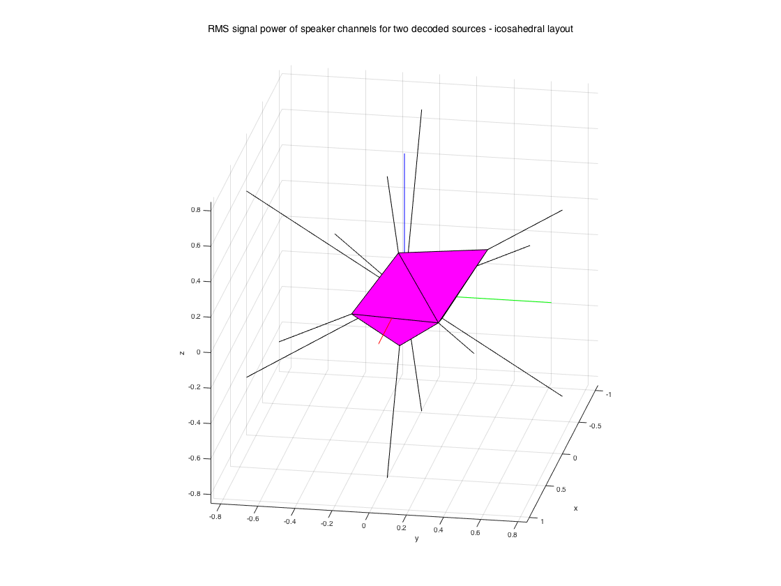
Encoding and decoding ambisonic signals is straightforward. The example below shows encoding two noise signals at two directions to 3rd-order HOA signals, and then decoding them at 84 uniformly arranged loudspeakers using an ALLRAD max-rE decoder.
% encode two signals of 5sec of noise, coming from the front and
% front-left-up
fs = 48000;
t = 5;
src_sig = randn(t*fs, 2);
src_dir = [0 0; 90 30];

order = 2;
hoasig = encodeHOA_N3D(order, src_sig, src_dir);

% define a 12-speaker uniform setup
[u12, ls_dirs12_rad, mesh12] = platonicSolid('icosahedron');
ls_dirs12 = ls_dirs12_rad*180/pi;
% get ALLRAD decoder
MAXRE_ON = 1;
D_allrad12 = ambiDecoder(ls_dirs12, 'allrad', MAXRE_ON, order);

% decode signals
lssig = decodeHOA_N3D(hoasig, D_allrad12);
% alternatively
% lssig = hoasig * D_allrad12.';

% plot RMS distribution of the decoded signals, along speaker directions
Psig = sqrt(mean(lssig.^2)).';
Sx = zeros(2,12); Sx(2,:) = u12(:,1); % speaker lines
Sy = zeros(2,12); Sy(2,:) = u12(:,2); % speaker lines
Sz = zeros(2,12); Sz(2,:) = u12(:,3); % speaker lines
figure
patch('vertices', mesh12.vertices .* (Psig*ones(1,3)), 'faces', mesh12.faces, 'facecolor', 'm')
line([0 1.5*max(Psig)],[0 0],[0 0],'color','r') % axis lines
line([0 0],[0 1.5*max(Psig)],[0 0],'color','g') % axis lines
line([0 0],[0 0],[0 1.5*max(Psig)],'color','b') % axis lines
line(Sx,Sy,Sz,'color','k') % plot speakers
axis equal
xlabel('x'), ylabel('y'), zlabel('z'), grid, view(100,20)
h = gcf; h.Position(3:4) = 2*h.Position(3:4);
suptitle('RMS signal power of speaker channels for two decoded sources - icosahedral layout')
FREQUENCY DEPENDENT-DECODING
When HOA-encoded sound scenes are used, like in the previous example, the HOA signals are broadband and frequency considerations depend only on the reproduction side. A common approach is to use an amplitude preserving unweighted decoder at low frequencies, with a cutoff frequency between 400~700Hz depending on the room, and an energy preserving max-rE weighted decoder at higher frequencies (termed dual-band decoding in ambisonic slang).
Decoding ambisonic recordings, however, captured with some spherical microphone array, is more complicated because the HOA signals themselves become frequency-dependent due to the microphone array properties. This is not very obvious with 1st-order signals (B-format), but it becomes very pronounced for higher-orders. E.g. the Eigenmike array delivers 2nd-order signals above ~500Hz and 3rd-order signals above ~1300Hz. Using a single decoding matrix for all mid-high frequencies may sound ok and it's definitely the simplest solution, but technically there will be some loss of power and colouration for a source captured from some direction and then decoded, due to the decoding matrix tuned to preserve energy using all HOA signals. Since certain HOA signals vanish at certain ranges, an alternative approach is to use as many decoding matrices as HOA frequency ranges, e.g. for the Eigenmike case: an amplitude-preserving unweighted 1st-order decoder f<500Hz, an energy-preserving max-rE 2nd-order decoder 500Hz<f<1200Hz, an energy-preserving max-rE 3rd-order decoder 1200Hz<f.
Frequency dependent-decoding can be done using decodeHOA_N3D() function, and passing an additional argument specifying the cutoff frequencies for the HOA ranges. As many decoding matrices as ranges should be defined in this case. A filterbank is applied internally to split the signals, decode the different ranges and combine the speaker outputs.
% encode one noise signal of 5sec of noise, coming from the front
fs = 48000;
t = 5;
src_sig = randn(t*fs, 1);
src_dir = [0 0];
order = 3;
hoasig = encodeHOA_N3D(order, src_sig, src_dir);

% Dual-band decoding at a 20-speaker uniform setup
[~, ls_dirs20_rad] = platonicSolid('dodecahedron'); % dodecahedral setup
ls_dirs20 = ls_dirs20_rad*180/pi;
ls_num = size(ls_dirs20,1);
cutoff = 500;
order = 3;
D_low = ambiDecoder(ls_dirs20, 'mmd', 0, order);
D_high = ambiDecoder(ls_dirs20, 'allrad', 1, order);
D_dualband = cat(3, D_low, D_high);
y_dualband = decodeHOA_N3D(hoasig, D_dualband, cutoff, fs);

% Frequency/order-dependent decoding for the Eigenmike at a 20-speaker uniform setup
cutoffs = [500 1200];
max_order = 3;
D_eigen = zeros(ls_num,(max_order+1)^2, max_order);
% f<500Hz, 1st-order
D_eigen(:,1:2^2,1) = ambiDecoder(ls_dirs20, 'mmd', 0, 1);
% 500<f<1200Hz, 2nd-order
D_eigen(:,1:3^2,2) = ambiDecoder(ls_dirs20, 'allrad', 1, 2);
% 500<f<1200Hz, 3rd-order
D_eigen(:,1:4^2,3) = ambiDecoder(ls_dirs20, 'allrad', 1, 3);
y_eigen = decodeHOA_N3D(hoasig, D_eigen, cutoffs, fs);
ROTATION OF AMBISONIC SOUND SCENES (REQUIRES THE SHT-LIB)
Rotation of the HOA sound scene can be achieved with appropriate rotation matrices, designed directly in the spherical harmonic domain. Apart from the case of the B-format rotation, which corresponds directly to standard rotation matrices, HO rotation matrices can be computed through the more general spherical harmonic transform library by the author (see introduction above for the link).
After the library is added to the Matlab search path, rotations can be performed using the rotateHOA_N3D() function, specifying three angles on a yaw-pitch-roll convention.
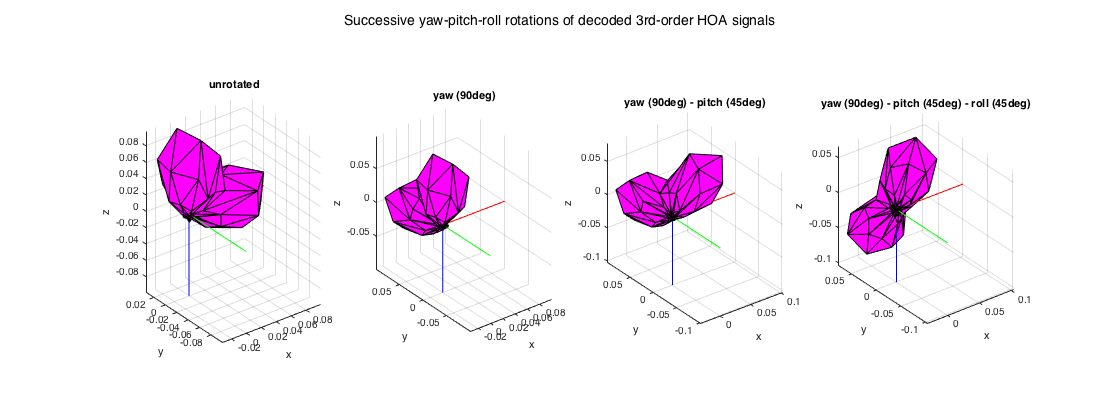
The following example encodes two sources to HOA signals, plots the decoding spatial power distribution, rotates the sound scene, and replots the rotated distribution.
% encode two signals of 5sec of noise, coming from the front and
% front-left-up
fs = 48000;
t = 5;
src_sig = randn(t*fs, 2);
src_dir = [0 0; 0 90];
order = 3;
hoasig = encodeHOA_N3D(order, src_sig, src_dir);
% rotate the sound scene, first around Z-axis by 90deg (yaw), then around
% the new Y'-axis by 45deg (pitch), then around the new X''-axis by 45deg
% (roll). Compute each step individually for plotting.
yaw = 90;
pitch = 45;
roll = 45;
hoasig_rot_y = rotateHOA_N3D(hoasig, yaw, 0, 0);
hoasig_rot_yp = rotateHOA_N3D(hoasig, yaw, pitch, 0);
hoasig_rot_ypr = rotateHOA_N3D(hoasig, yaw, pitch, roll);

% define an 84-speaker uniform setup
[u84, ls_dirs84_rad] = getTdesign(12);
ls_dirs84 = ls_dirs84_rad*180/pi;
mesh84.vertices = u84;
mesh84.faces = sphDelaunay(ls_dirs84_rad);
% get a sampling decoder
MAXRE_ON = 1;
D_sad84 = ambiDecoder(ls_dirs84, 'sad', MAXRE_ON, order);
% decode signals
LSsig84 = decodeHOA_N3D(hoasig, D_sad84);
% decode rotated signals
LSsig84_rot_y = decodeHOA_N3D(hoasig_rot_y, D_sad84);
LSsig84_rot_yp = decodeHOA_N3D(hoasig_rot_yp, D_sad84);
LSsig84_rot_ypr = decodeHOA_N3D(hoasig_rot_ypr, D_sad84);

% plot RMS power distribution of the decoded signals
Psig = sqrt(mean(LSsig84.^2)).';
figure
subplot(141)
patch('vertices', mesh84.vertices .* (Psig*ones(1,3)), 'faces', mesh84.faces, 'facecolor', 'm')
axis(max(Psig)*[-1 1 -1 1 -1 1]), axis equal
xlabel('x'), ylabel('y'), zlabel('z'), grid
line([0 max(Psig)],[0 0],[0 0],'color','r'), line([0 0],[0 -max(Psig)],[0 0],'color','g'), line([0 0],[0 0],[0 -max(Psig)],'color','b')
title('unrotated')
subplot(142)
Psig_rot = sqrt(mean(LSsig84_rot_y.^2)).';
patch('vertices', mesh84.vertices .* (Psig_rot*ones(1,3)), 'faces', mesh84.faces, 'facecolor', 'm')
axis(max(Psig)*[-1 1 -1 1 -1 1]), axis equal
xlabel('x'), ylabel('y'), zlabel('z'), grid
line([0 max(Psig_rot)],[0 0],[0 0],'color','r'), line([0 0],[0 -max(Psig_rot)],[0 0],'color','g'), line([0 0],[0 0],[0 -max(Psig_rot)],'color','b')
title('yaw (90deg)')
subplot(143)
Psig_rot = sqrt(mean(LSsig84_rot_yp.^2)).';
patch('vertices', mesh84.vertices .* (Psig_rot*ones(1,3)), 'faces', mesh84.faces, 'facecolor', 'm')
axis(max(Psig)*[-1 1 -1 1 -1 1]), axis equal
xlabel('x'), ylabel('y'), zlabel('z'), grid
line([0 max(Psig_rot)],[0 0],[0 0],'color','r'), line([0 0],[0 -max(Psig_rot)],[0 0],'color','g'), line([0 0],[0 0],[0 -max(Psig_rot)],'color','b')
title('yaw (90deg) - pitch (45deg)')
subplot(144)
Psig_rot = sqrt(mean(LSsig84_rot_ypr.^2)).';
patch('vertices', mesh84.vertices .* (Psig_rot*ones(1,3)), 'faces', mesh84.faces, 'facecolor', 'm')
axis(max(Psig)*[-1 1 -1 1 -1 1]), axis equal
xlabel('x'), ylabel('y'), zlabel('z'), grid
line([0 max(Psig_rot)],[0 0],[0 0],'color','r'), line([0 0],[0 -max(Psig_rot)],[0 0],'color','g'), line([0 0],[0 0],[0 -max(Psig_rot)],'color','b')
title('yaw (90deg) - pitch (45deg) - roll (45deg)'), view(3)
h = gcf; h.Position(3) = 2*h.Position(3);
suptitle('Successive yaw-pitch-roll rotations of decoded 3rd-order HOA signals')
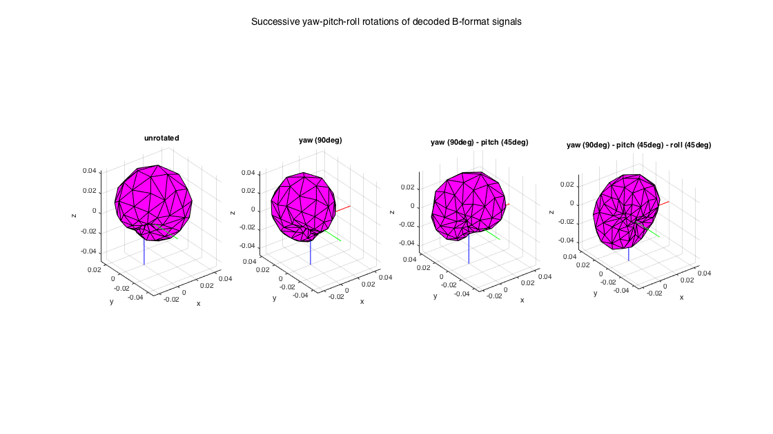
B-format rotation requires just a regular rotation matrix, for this case use the rotateBformat() function. The example below duplicates the above HOA case, but doing everything with the traditional 1st-order B-format.
% encode two signals of 5sec of noise, coming from the front and
% front-left-up
fs = 48000;
t = 5;
src_sig = randn(t*fs, 2);
src_dir = [0 0; 0 90];
bfsig = encodeBformat(src_sig, src_dir);
% rotate the sound scene, first around Z-axis by 90deg (yaw), then around
% the new Y'-axis by 45deg (pitch), then around the new X''-axis by 45deg
% (roll). Compute each step individually for plotting.
yaw = 90;
pitch = 45;
roll = 45;
bfsig_rot_y = rotateBformat(bfsig, yaw, 0, 0);
bfsig_rot_yp = rotateBformat(bfsig, yaw, pitch, 0);
bfsig_rot_ypr = rotateBformat(bfsig, yaw, pitch, roll);

% decode signals
LSsig84 = decodeBformat(bfsig, D_sad84);
% decode rotated signals
LSsig84_rot_y = decodeBformat(bfsig_rot_y, D_sad84);
LSsig84_rot_yp = decodeBformat(bfsig_rot_yp, D_sad84);
LSsig84_rot_ypr = decodeBformat(bfsig_rot_ypr, D_sad84);

% plot RMS power distribution of the decoded signals
Psig = sqrt(mean(LSsig84.^2)).';
figure
subplot(141)
patch('vertices', mesh84.vertices .* (Psig*ones(1,3)), 'faces', mesh84.faces, 'facecolor', 'm')
axis(max(Psig)*[-1 1 -1 1 -1 1]), axis equal, grid
xlabel('x'), ylabel('y'), zlabel('z')
line([0 max(Psig)],[0 0],[0 0],'color','r'), line([0 0],[0 -max(Psig)],[0 0],'color','g'), line([0 0],[0 0],[0 -max(Psig)],'color','b')
title('unrotated')
subplot(142)
Psig_rot = sqrt(mean(LSsig84_rot_y.^2)).';
patch('vertices', mesh84.vertices .* (Psig_rot*ones(1,3)), 'faces', mesh84.faces, 'facecolor', 'm')
axis(max(Psig)*[-1 1 -1 1 -1 1]), axis equal, grid
xlabel('x'), ylabel('y'), zlabel('z')
line([0 max(Psig_rot)],[0 0],[0 0],'color','r'), line([0 0],[0 -max(Psig_rot)],[0 0],'color','g'), line([0 0],[0 0],[0 -max(Psig_rot)],'color','b')
title('yaw (90deg)')
subplot(143)
Psig_rot = sqrt(mean(LSsig84_rot_yp.^2)).';
patch('vertices', mesh84.vertices .* (Psig_rot*ones(1,3)), 'faces', mesh84.faces, 'facecolor', 'm')
axis(max(Psig)*[-1 1 -1 1 -1 1]), axis equal, grid
xlabel('x'), ylabel('y'), zlabel('z')
line([0 max(Psig_rot)],[0 0],[0 0],'color','r'), line([0 0],[0 -max(Psig_rot)],[0 0],'color','g'), line([0 0],[0 0],[0 -max(Psig_rot)],'color','b')
title('yaw (90deg) - pitch (45deg)')
subplot(144)
Psig_rot = sqrt(mean(LSsig84_rot_ypr.^2)).';
patch('vertices', mesh84.vertices .* (Psig_rot*ones(1,3)), 'faces', mesh84.faces, 'facecolor', 'm')
axis(max(Psig)*[-1 1 -1 1 -1 1]), axis equal, grid
xlabel('x'), ylabel('y'), zlabel('z')
line([0 max(Psig_rot)],[0 0],[0 0],'color','r'), line([0 0],[0 -max(Psig_rot)],[0 0],'color','g'), line([0 0],[0 0],[0 -max(Psig_rot)],'color','b')
title('yaw (90deg) - pitch (45deg) - roll (45deg)')
h = gcf; h.Position(3) = 2*h.Position(3); h.Position(4) = 1.5*h.Position(4);
suptitle('Successive yaw-pitch-roll rotations of decoded B-format signals')
CONVERSION BETWEEN DIFFERENT FORMATS
All the HOA processing here assumes orthonormal real SHs, for the exact convention's details check the code of getRSH() or the documentation of the SHT-lib. Furthermore, indexing of HOA channels and SHs follows the rational single number indexing of SH components found in all other fields. These two conventions correspond to N3D normalization and ACN channel indexing in ambisonic slang. There are a few functions in the library that convert between these and two other common conventions - in case you obtain signals following them, you can use these functions to convert them to N3D_ACN and apply the operations of the library. Similarly, you can convert back to these other conventions if you need to share HOA signals in that format for any reason. One can convert from N3D to the Schmidt semi-normalization (SN3D), and back, and one can convert from the ACN channel indexing to the SID (see [ref.11]) indexing and back.
% N3D to SN3D and back
hoa_N3D_ACN = encodeHOA_N3D(3, 1, [0 0]);
hoa_SN3D_ACN = convert_N3D_SN3D(hoa_N3D_ACN, 'n2sn');
hoa_N3D_ACN_2 = convert_N3D_SN3D(hoa_SN3D_ACN, 'sn2n');

% ACN to SID and back
hoa_N3D_SID = convert_ACN_SID(hoa_N3D_ACN, 'acn2sid');
hoa_N3D_ACN_3 = convert_ACN_SID(hoa_N3D_SID, 'sid2acn');

% ACN to Bformat (1st-order only) and back. Here the sqrt(2) factor of the
% B-format is assumed to be on the dipoles.
foa_N3D_ACN = encodeHOA_N3D(1, 1, [0 0]);
bf = convert_N3D_Bformat(foa_N3D_ACN, 'n2b');
foa_N3D_ACN_2 = convert_N3D_Bformat(bf, 'b2n');
REFERENCES
[1] Zotter, F., Pomberger, H., Noisternig, M. (2012). Energy-Preserving Ambisonic Decoding. Acta Acustica United with Acustica, 98(1), 37?47.
[2] Zotter, F., Frank, M. (2012). All-Round Ambisonic Panning and Decoding. Journal of the Audio Engineering Society, 60(10), 807?820.
[3] Epain, N., Jin, C. T., Zotter, F. (2014). Ambisonic Decoding With Constant Angular Spread. Acta Acustica United with Acustica, 100, 928?936.
[4] Daniel, J. (2001). Repr?sentation de champs acoustiques, application ? la transmission et ? la reproduction de sc?nes sonores complexes dans un contexte multim?dia. Doctoral Thesis. Universit? Paris 6.
[5] Makita, Y. (1962). On the directional localization of sound in the stereophonic sound field. EBU Review, 73, 1536?1539.
[6] Gerzon, M. A. (1992). General Metatheory of Auditory Localization. In 92nd AES Convention (Preprint 3306). Vienna, Austria.
[7] Merimaa, J. (2007). Energetic sound field analysis of stereo and multichannel loudspeaker reproduction. In 123rd AES Convention. New York, NY.
[8] Matthias, F. (2013). Phantom Sources using Multiple Loudspeakers in the Horizontal Plane. Doctoral thesis, Institute of Electronic Music and Acoustics, University of Music and Performing Arts, Graz
[9] Laitinen, M., Vilkamo, J., Jussila, K., Politis, A., & Pulkki, V. (2014). Gain normalization in amplitude panning as a function of frequency and room reverberance. In 55th International Conference of AES. Helsinki, Finland.
[10] Frank, M. (2013). Source Width of Frontal Phantom Sources: Perception, Measurement, and Modeling. Archives of Acoustics. 38(3), 311?319
[11] Daniel, J. (2003). Spatial Sound Encoding Including Near Field Effect : Introducing Distance Coding Filters and a Viable , New Ambisonic Format. In 23rd International Conference of AES. Copenhagen, Denmark.