SENSOR ARRAY RESPONSE SIMULATOR

ARRAYS OF OMNIDIRECTIONAL MICROPHONES
ARRAY OF DIRECTIONAL MICROPHONES
ARRAY OF HIGHER ORDER DIRECTIONAL MICROPHONES
ARRAY OF MICROPHONES ON A CYLINDRICAL/SPHERICAL SCATTERER
ARRAY OF MICROPHONES AT A DISTANCE FROM A CYLINDRICAL/SPHERICAL SCATTERER
3D UNIFORM SPHERICAL ARRAY EXAMPLE
REFERENCES

%%%%%%%%%%%%%%%%%%%%%%%%%%%%%%%%%%%%%%%%%%%%%%%%%%%%%%%%%%%%%%%%%%%%%%%%%%%%
%
%   Archontis Politis, 2015
%   Department of Signal Processing and Acoustics, Aalto University, Finland
%   archontis.politis@aalto.fi
%
%%%%%%%%%%%%%%%%%%%%%%%%%%%%%%%%%%%%%%%%%%%%%%%%%%%%%%%%%%%%%%%%%%%%%%%%%%%%

This is a collection of MATLAB routines for simulation of array responses of

a) directional sensors and,

b) sensors mounted on, or at a distance from, a rigid spherical/cylindrical scatterer.

The computation of their frequency and impulse responses is based on the theoretical expansion of a scalar incident plane wave field to a series of wavenumber-dependent Bessel-family functions and direction-dependent Fourier or Legendre functions.

Alternatively, a function for arbitrary open arrays of directional microphones is included, not based on the expansion but directly on the steering vector formula of inter-sensor delays and sensor gains for user-defined directional patterns (e.g. arrays of cardioid microphones).

For more information on the expansions, you can have a look on [ref.1] and [ref.2]

and for example on http://en.wikipedia.org/wiki/Plane_wave_expansion and http://en.wikipedia.org/wiki/Jacobi-Anger_expansion

For any questions, comments, corrections, or general feedback, please contact archontis.politis@aalto.fi

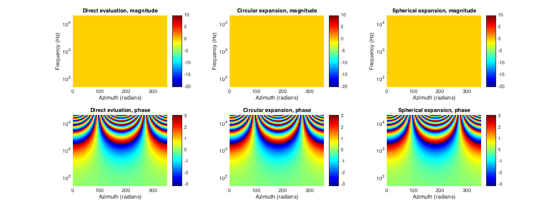
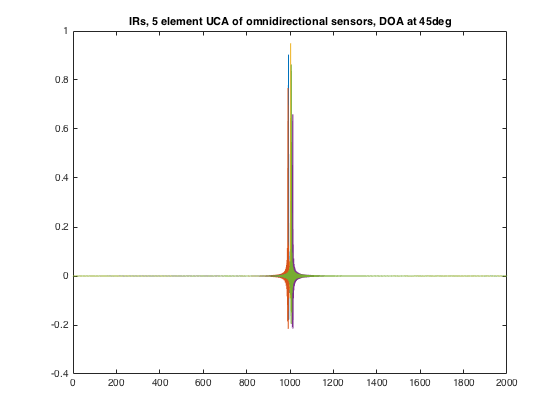
ARRAYS OF OMNIDIRECTIONAL MICROPHONES

This is the simplest case and the array responses can be computed either by simulateCylArray() for 2D, simulateSphArray() for 3D, or getArrayResponse() for both. Since getArrayResponse does not involve a spherical or cylindrical expansion, it is the easiest to use in this case.

% a uniform circular array of 5 elements at 10cm radius
mic_azi = (0:360/5:360-360/5)'*pi/180;
mic_elev = zeros(size(mic_azi));
R = 0.1;
[R_mic(:,1), R_mic(:,2), R_mic(:,3)] = sph2cart(mic_azi, mic_elev, R);

% plane wave direcitons to evaluate response
doa_azi = (0:5:355)'*pi/180;
doa_elev = zeros(size(doa_azi));
[U_doa(:,1), U_doa(:,2), U_doa(:,3)] = sph2cart(doa_azi, doa_elev, 1);

% impulse response parameters
fs = 40000;
Lfilt = 2000;
% simulate array using getArrayResponse()
fDirectivity = @(angle) 1; % response of omnidirectional microphone
[h_mic1, H_mic1] = getArrayResponse(U_doa, R_mic, [], fDirectivity, Lfilt, fs); % microphone orientation irrelevant in this case

% simulate array using 2D propagation and cylindrical expansion
N_order = 40; % order of expansion
[h_mic2, H_mic2] = simulateCylArray(Lfilt, mic_azi, doa_azi, 'open', R, N_order, fs);

% simulate array using 3D propagation and spherical expansion
[h_mic3, H_mic3] = simulateSphArray(Lfilt, [mic_azi mic_elev], [doa_azi doa_elev], 'open', R, N_order, fs);

% Plots
Nfft = Lfilt;
f = (0:Nfft/2)*fs/Nfft;

figure
subplot(231)
surf(doa_azi*180/pi, f, 20*log10(abs(squeeze(H_mic1(:,1,:)))))
view(2)
shading flat
set(gca,'yscale','log')
axis([0 355 50 20000])
caxis([-20 10]), colorbar, colormap(jet)
ylabel('Frequency (Hz)')
xlabel('Azimuth (radians)')
title('Direct evaluation, magnitude')
subplot(234)
surf(doa_azi*180/pi, f, angle(squeeze(H_mic1(:,1,:))))
view(2)
shading flat
set(gca,'yscale','log')
axis([0 355 50 20000])
colorbar
xlabel('Azimuth (radians)')
title('Direct evluation, phase')
subplot(232)
surf(doa_azi*180/pi, f, 20*log10(abs(squeeze(H_mic2(:,1,:)))))
view(2)
shading flat
set(gca,'yscale','log')
axis([0 355 50 20000])
caxis([-20 10]), colorbar, colormap(jet)
ylabel('Frequency (Hz)')
xlabel('Azimuth (radians)')
title('Circular expansion, magnitude')
subplot(235)
surf(doa_azi*180/pi, f, angle(squeeze(H_mic2(:,1,:))))
view(2)
shading flat
set(gca,'yscale','log')
axis([0 355 50 20000])
colorbar
xlabel('Azimuth (radians)')
title('Circular expansion, phase')
subplot(233)
surf(doa_azi*180/pi, f, 20*log10(abs(squeeze(H_mic3(:,1,:)))))
view(2)
shading flat
set(gca,'yscale','log')
axis([0 355 50 20000])
caxis([-20 10]), colorbar, colormap(jet)
ylabel('Frequency (Hz)')
xlabel('Azimuth (radians)')
title('Spherical expansion, magnitude')
subplot(236)
surf(doa_azi*180/pi, f, angle(squeeze(H_mic3(:,1,:))))
view(2)
shading flat
set(gca,'yscale','log')
axis([0 355 50 20000])
colorbar
xlabel('Azimuth (radians)')
title('Spherical expansion, phase')
h = gcf; h.Position(3) = 2*h.Position(3);

% plot the array impulse responses for all microphones and doa at 45deg
figure
plot(squeeze(h_mic1(:,:,45/5+1)))
title('IRs, 5 element UCA of omnidirectional sensors, DOA at 45deg')

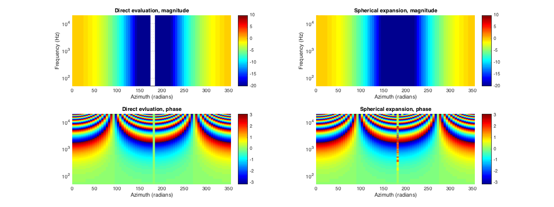
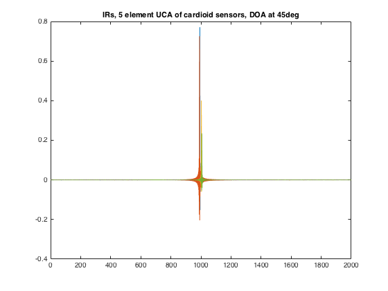
ARRAY OF DIRECTIONAL MICROPHONES

Simulate the same case but for first-order directional microphones instead of omnidirectional ones. These can be evaluated using the getArrayResponse() or by spherical expansion using simulateSphArray(). At the moment circular expansion of directional microphones is not included, and since there are two ways already to compute, it's probably not needed.

% first-order directivity coefficient, a + (1-a)cos(theta)
% for a = 1, same as the previous omnidirectional case above
a = 0.5; % cardioid response

% simulate array using getArrayResponse()
fDirectivity = @(angle) a + (1-a)*cos(angle); % response for cardioid microphone
[h_mic1, H_mic1] = getArrayResponse(U_doa, R_mic, [], fDirectivity, Lfilt, fs); % microphone orientation radial

% simulate array using spherical expansion
arrayType = 'directional';
[h_mic2, H_mic2] = simulateSphArray(Lfilt, [mic_azi mic_elev], [doa_azi doa_elev], arrayType, R, N_order, fs, a);

% Plots
figure
subplot(221)
surf(doa_azi*180/pi, f, 20*log10(abs(squeeze(H_mic1(:,1,:)))))
view(2)
shading flat
set(gca,'yscale','log')
axis([0 355 50 20000])
caxis([-20 10]), colorbar, colormap(jet)
ylabel('Frequency (Hz)')
xlabel('Azimuth (radians)')
title('Direct evaluation, magnitude')
subplot(223)
surf(doa_azi*180/pi, f, angle(squeeze(H_mic1(:,1,:))))
view(2)
shading flat
set(gca,'yscale','log')
axis([0 355 50 20000])
colorbar
xlabel('Azimuth (radians)')
title('Direct evluation, phase')
subplot(222)
surf(doa_azi*180/pi, f, 20*log10(abs(squeeze(H_mic2(:,1,:)))))
view(2)
shading flat
set(gca,'yscale','log')
axis([0 355 50 20000])
caxis([-20 10]), colorbar, colormap(jet)
ylabel('Frequency (Hz)')
xlabel('Azimuth (radians)')
title('Spherical expansion, magnitude')
subplot(224)
surf(doa_azi*180/pi, f, angle(squeeze(H_mic2(:,1,:))))
view(2)
shading flat
set(gca,'yscale','log')
axis([0 355 50 20000])
colorbar
xlabel('Azimuth (radians)')
title('Spherical expansion, phase')
h = gcf; h.Position(3) = 2*h.Position(3);

% plot the array impulse responses for all microphones and doa at 45deg
figure
plot(squeeze(h_mic1(:,:,45/5+1)))
title('IRs, 5 element UCA of cardioid sensors, DOA at 45deg')

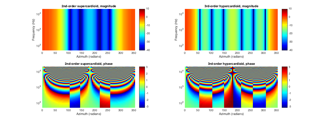
ARRAY OF HIGHER ORDER DIRECTIONAL MICROPHONES

Higher-order directional patterns can be simulated using getArrayResponse(). Appropriate functions should be defined, and different patterns can be passed for each element of the array. Not that this approach will ignore the frequency dependency that occurs in practice with the acoustical processing generating these higher-order patterns. For proper response modeling in such cases, one can simulate the response of the elements of the subarray, and apply the associated processing for pattern generation to the resulting IRs (see e.g. [ref.3]).

% define an array of two differential patterns, one 2nd-order supercardioid
% and a 3rd-order hypercardioid, oriented at front and at 10cm distance
% between (weights from [ref.3])
a2_scard = [(3 - sqrt(7))/4; (3*sqrt(7) - 7)/2; (15 - (5*sqrt(7)))/4];
a3_hcard = [-3/32; -15/32; 15/32; 35/32];
fDir1 = @(angle) a2_scard(1) + a2_scard(2)*cos(angle) + a2_scard(3)*cos(angle).^2;
fDir2 = @(angle) a3_hcard(1) + a3_hcard(2)*cos(angle) + a3_hcard(3)*cos(angle).^2 + a3_hcard(4)*cos(angle).^3;
fDirHandles{1} = fDir1;
fDirHandles{2} = fDir2;
R_mic = 0.5*[0 1 0; 0 -1 0];
U_orient = [1 0 0; 1 0 0];

% simulate array using getArrayResponse()
[~, H_mic] = getArrayResponse(U_doa, R_mic, U_orient, fDirHandles, Lfilt, fs);

% Plots
figure
subplot(221)
surf(doa_azi*180/pi, f, 20*log10(abs(squeeze(H_mic(:,1,:)))))
view(2)
shading flat
set(gca,'yscale','log')
axis([0 355 50 20000])
caxis([-40 10]), colorbar, colormap(jet)
ylabel('Frequency (Hz)')
xlabel('Azimuth (radians)')
title('2nd-order supercardioid, magnitude')
subplot(223)
surf(doa_azi*180/pi, f, angle(squeeze(H_mic(:,1,:))))
view(2)
shading flat
set(gca,'yscale','log')
axis([0 355 50 20000])
colorbar
xlabel('Azimuth (radians)')
title('2nd-order supercardioid, phase')
subplot(222)
surf(doa_azi*180/pi, f, 20*log10(abs(squeeze(H_mic(:,2,:)))))
view(2)
shading flat
set(gca,'yscale','log')
axis([0 355 50 20000])
caxis([-40 10]), colorbar, colormap(jet)
ylabel('Frequency (Hz)')
xlabel('Azimuth (radians)')
title('3rd-order hypercardioid, magnitude')
subplot(224)
surf(doa_azi*180/pi, f, angle(squeeze(H_mic(:,2,:))))
view(2)
shading flat
set(gca,'yscale','log')
axis([0 355 50 20000])
colorbar
xlabel('Azimuth (radians)')
title('3rd-order hypercardioid, phase')
h = gcf; h.Position(3) = 2*h.Position(3);

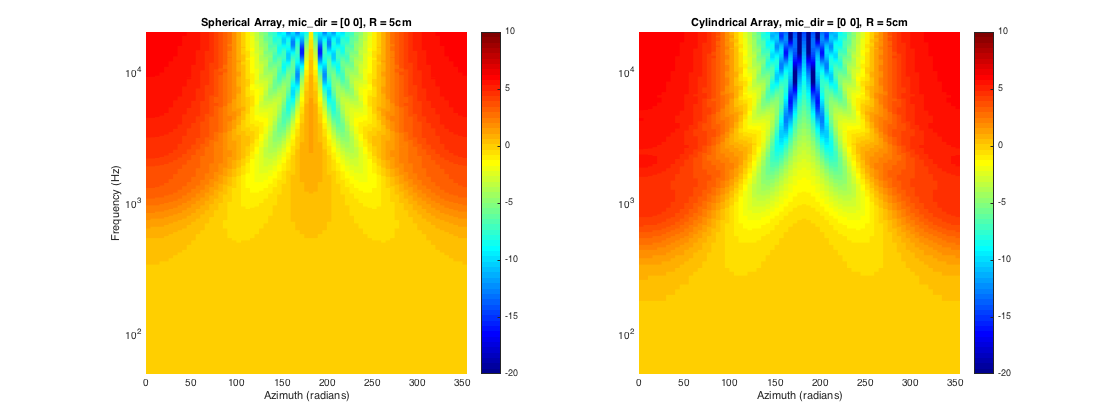
ARRAY OF MICROPHONES ON A CYLINDRICAL/SPHERICAL SCATTERER

Microphones mounted on a spherical scatterer (for 3D processing), or on a cylindrical scatterer (for 2D processing) exhibit some advantages over open arrays of omnidirectional microphones, mainly due to the inherent directionality of the scattering body, and the fact that they are more suitable for working in the spatial Fourier transform domain (also known as eigenbeam processing, or phase-mode processing in the literature) in which case the open array exhibits resonant frequencies for which the transformed signals vanish.

The response of a plane wave scattered by these fundamental geometries is known analytically, and it involves the special functions and their derivatives, included in the library.

% Simulate a single microphone mounted on a cylinder and on a sphere of radius 5cm
R = 0.05;
arrayType = 'rigid';
N_order = 40; % order of expansion
mic_azi = 0;
mic_dir = [0 0];

% Compute simulated impulse responses
doa_azi = (0:5:355)'*pi/180;
doa_dirs = [doa_azi zeros(size(doa_azi))];
[~, H_mic_cyl] = simulateCylArray(Lfilt, mic_azi, doa_azi, arrayType, R, N_order, fs);
[~, H_mic_sph] = simulateSphArray(Lfilt, mic_dir, doa_dirs, arrayType, R, N_order, fs);

% plots
figure
subplot(121)
surf(doa_azi*180/pi, f, 20*log10(abs(squeeze(H_mic_sph(:,1,:)))))
view(2)
shading flat
set(gca,'yscale','log')
axis([0 355 50 20000])
caxis([-20 10]), colorbar, colormap(jet)
ylabel('Frequency (Hz)')
xlabel('Azimuth (radians)')
title('Spherical Array, mic\_dir = [0 0], R = 5cm')
subplot(122)
surf(doa_azi*180/pi, f, 20*log10(abs(squeeze(H_mic_cyl(:,1,:)))))
view(2)
shading flat
set(gca,'yscale','log')
axis([0 355 50 20000])
caxis([-20 10]), colorbar, colormap(jet)
xlabel('Azimuth (radians)')
title('Cylindrical Array, mic\_dir = [0 0], R = 5cm')
h = gcf; h.Position(3) = 2*h.Position(3);

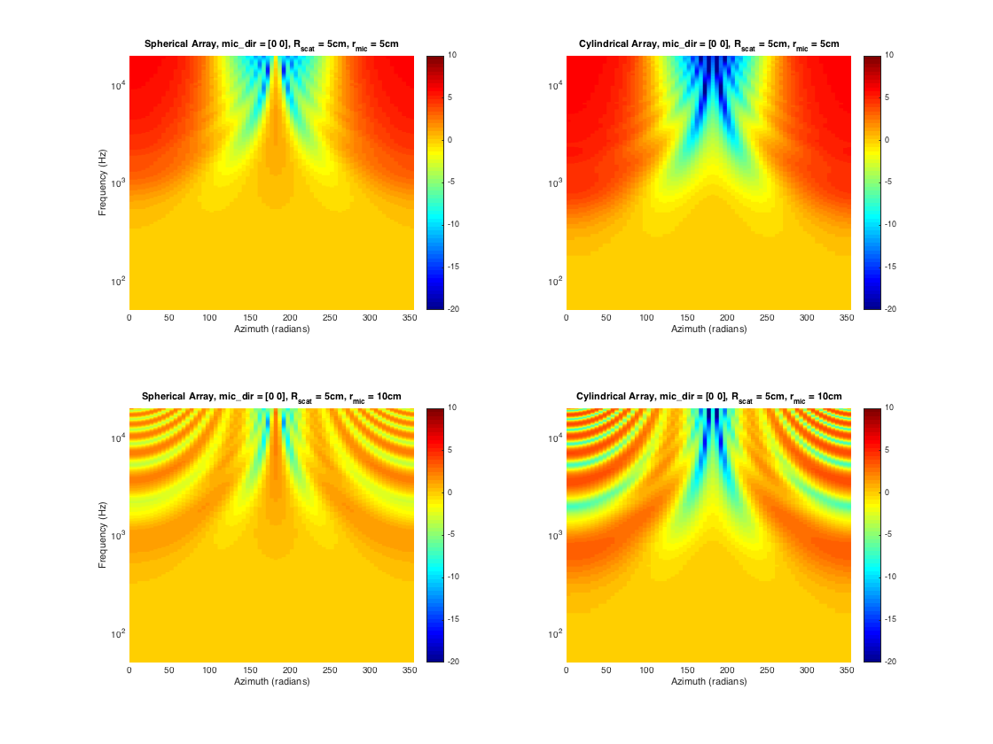
ARRAY OF MICROPHONES AT A DISTANCE FROM A CYLINDRICAL/SPHERICAL SCATTERER

Apart from the functions that evaluate the responses on the surface of a scatterer, functions are included that evaluate the response at some distance away from the scatterer, for which the effect gradually diminishes with distance. This case may be useful for example in simulating arrays that place microphones at different radii for broadband eigenbeam processing, or for simulating a hearing aid array from some small distance of a spherical head.

% Simulate a microphone mounted on a cylinder and on a sphere of radius
% 5cm, and a second microphone at 5cm distance from the scatterer
R = 0.05;
N_order = 40; % order of expansion
mic_azi = 0;
mic_elev = 0;
mic_dirs_sph = [mic_azi mic_elev R; mic_azi mic_elev 2*R];
mic_dirs_cyl = [mic_azi R; mic_azi 2*R];

% Compute simulated impulse responses
doa_azi = (0:5:355)'*pi/180;
doa_dirs = [doa_azi zeros(size(doa_azi))];

[~, H_mic_cyl] = cylindricalScatterer(mic_dirs_cyl, doa_azi, R, N_order, Lfilt, fs);
[~, H_mic_sph] = sphericalScatterer(mic_dirs_sph, doa_dirs, R, N_order, Lfilt, fs);

% plots
figure
subplot(221)
surf(doa_azi*180/pi, f, 20*log10(abs(squeeze(H_mic_sph(:,1,:)))))
view(2)
shading flat
set(gca,'yscale','log')
axis([0 355 50 20000])
caxis([-20 10]), colorbar, colormap(jet)
ylabel('Frequency (Hz)')
xlabel('Azimuth (radians)')
title('Spherical Array, mic\_dir = [0 0], R_{scat} = 5cm, r_{mic} = 5cm')
subplot(222)
surf(doa_azi*180/pi, f, 20*log10(abs(squeeze(H_mic_cyl(:,1,:)))))
view(2)
shading flat
set(gca,'yscale','log')
axis([0 355 50 20000])
caxis([-20 10]), colorbar, colormap(jet)
xlabel('Azimuth (radians)')
title('Cylindrical Array, mic\_dir = [0 0], R_{scat} = 5cm, r_{mic} = 5cm')
subplot(223)
surf(doa_azi*180/pi, f, 20*log10(abs(squeeze(H_mic_sph(:,2,:)))))
view(2)
shading flat
set(gca,'yscale','log')
axis([0 355 50 20000])
caxis([-20 10]), colorbar, colormap(jet)
ylabel('Frequency (Hz)')
xlabel('Azimuth (radians)')
title('Spherical Array, mic\_dir = [0 0], R_{scat} = 5cm, r_{mic} = 10cm')
subplot(224)
surf(doa_azi*180/pi, f, 20*log10(abs(squeeze(H_mic_cyl(:,2,:)))))
view(2)
shading flat
set(gca,'yscale','log')
axis([0 355 50 20000])
caxis([-20 10]), colorbar, colormap(jet)
xlabel('Azimuth (radians)')
title('Cylindrical Array, mic\_dir = [0 0], R_{scat} = 5cm, r_{mic} = 10cm')
h = gcf; h.Position(3:4) = 2*h.Position(3:4);

3D UNIFORM SPHERICAL ARRAY EXAMPLE

Simulate a uniform spherical array with the specifications of the Eigenmike array, suitable for up to 4th-order eigenbeam processing

% Eigenmike angles, in [azimuth, elevation] form
mic_dirs = ...
    [0    21;
    32     0;
     0   -21;
   328     0;
     0    58;
    45    35;
    69     0;
    45   -35;
     0   -58;
   315   -35;
   291     0;
   315    35;
    91    69;
    90    32;
    90   -31;
    89   -69;
   180    21;
   212     0;
   180   -21;
   148     0;
   180    58;
   225    35;
   249     0;
   225   -35;
   180   -58;
   135   -35;
   111     0;
   135    35;
   269    69;
   270    32;
   270   -32;
   271   -69];
mic_dirs_rad = mic_dirs*pi/180;

% Eigenmike radius
R = 0.042;

% Type and order of approximation
arrayType = 'rigid';
N_order = 30;

% Obtain responses for front, side and up DOAs
src_dirs_rad = [0 0; pi 0; 0 pi/2];
[h_mic, H_mic] = simulateSphArray(Lfilt, mic_dirs_rad, src_dirs_rad, arrayType, R, N_order, fs);

REFERENCES

[1] Earl G. Williams, "Fourier Acoustics: Sound Radiation and Nearfield Acoustical Holography", Academic Press, 1999

[2] Heinz Teutsch, "Modal Array Signal Processing: Principles and Applications of Acoustic Wavefield Decomposition", Springer, 2007

[3] Elko, W. Gary, "Differential Microphone Arrays", In Y. Huang & J. Benesty (Eds.), Audio signal processing for next-generation multimedia communication systems (pp. 11?65). Springer, 2004