ACOUSTICAL SPHERICAL ARRAY PROCESSING LIBRARY
Contents
- MICROPHONE SIGNALS TO SH SIGNALS
- ---Theory based-filters
- ---Measurement based-filters
- SIGNAL-INDEPENDENT BEAMFORMING IN THE SPHERICAL HARMONIC DOMAIN
- ---Cardioids
- ---Hypercardioids (regular spherical beamformer, plane-wave decomposition, superdirective, or max-DI)
- ---Supercardioids (max front-to-back power ratio)
- ---Max-EV (energy vector) patterns
- ---Dolph-Chebyshev beampatterns
- ---Differential arrays
- ---Arbitrary beampatterns
- ---Weighted velocity beamformers
- SIGNAL-DEPENDENT AND PARAMETRIC BEAMFORMING
- ---Plane-wave decomposition beamformer with null-steering
- ---Nullformer for diffuse sound extraction
- ---MVDR
- ---LCMV
- ---iPMMW
- DIRECTION-OF-ARRIVAL (DoA) ESTIMATION IN THE SHD
- ---Plane-wave decomposition power map
- ---MVDR power map
- ---MUSIC spectrum
- ---Intensity vector DoA estimation
- DIFFUSENESS AND DIRECT-TO-DIFFUSE RATIO (DDR) ESTIMATION
- ---Sigle source case
- ---Multiple sources case
- DIFFUSE-FIELD COHERENCE OF DIRECTIONAL SENSORS/BEAMFORMERS [ref.8]
- ---DFC between two coincident beamformers/sensors
- ---DFC matrix of microphones on sphere
- ---DFC between spaced directional sensors with arbitrary directivity
- REFERENCES
%%%%%%%%%%%%%%%%%%%%%%%%%%%%%%%%%%%%%%%%%%%%%%%%%%%%%%%%%%%%%%%%%%%%%%%%%%%%
%
%   Archontis Politis, 2016
%   Department of Signal Processing and Acoustics, Aalto University, Finland
%   archontis.politis@aalto.fi
%
%%%%%%%%%%%%%%%%%%%%%%%%%%%%%%%%%%%%%%%%%%%%%%%%%%%%%%%%%%%%%%%%%%%%%%%%%%%%
This is a collection MATLAB routines that perform array processing techniques on spatially transformed signals, commonly captured with a spherical microphone array. The routines fall into four main categories:
a) obtain spherical harmonic (SH) signals with broadband characteristics, as much as possible,
b) generate beamforming weights in the spherical harmonic domain (SHD) for common signal-independent beampatterns,
c) demonstrate some adaptive beamforming methods in the SHD,
d) demonstrate some direction-of-arrival (DoA) estimation methods in the SHD,
e) demonstrate methods for analysis of diffuseness in the sound-field
f) demonstrate flexible diffuse-field coherence modeling of arrays
The latest version of the library can be found at
https://github.com/polarch/Spherical-Array-Processing
Detailed demonstration of the routines is given in TEST_SCRIPTS.m and at
http://research.spa.aalto.fi/projects/spharrayproc-lib/spharrayproc.html
The library relies in the other two libraries of the author related to acoustical array processing found at:
https://github.com/polarch/Array-Response-Simulator
https://github.com/polarch/Spherical-Harmonic-Transform
They need to be added to the MATLAB path for most functions to work.
For any questions, comments, corrections, or general feedback, please contact archontis.politis@aalto.fi
MICROPHONE SIGNALS TO SH SIGNALS
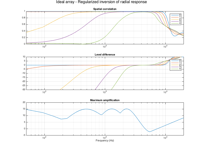
The first operation is to obtain the SH signals from the microphone signals. That corresponds to two operations: a matrixing of the signals that performs a discrete spherical harmonic transform (SHT) on the sound pressure over the spherical array, followed by an equalization step of the SH signals that extrapolates them from the finite array radius to array-independent sound-field coefficients. This operation is limited by physical considerations, and the inversion should be limited to avoid excessive noise amplification in the SH signals. A few approaches are demonstrated below.
---Theory based-filters
The simplest approach avoids the effect of spatial aliasing and takes into account only the array radius [ref1]. An amplification limit has to be specified for the filters realizing this single-channel regularized inversion, which determines the amount of regularization needed in order not to exceed this threshold.
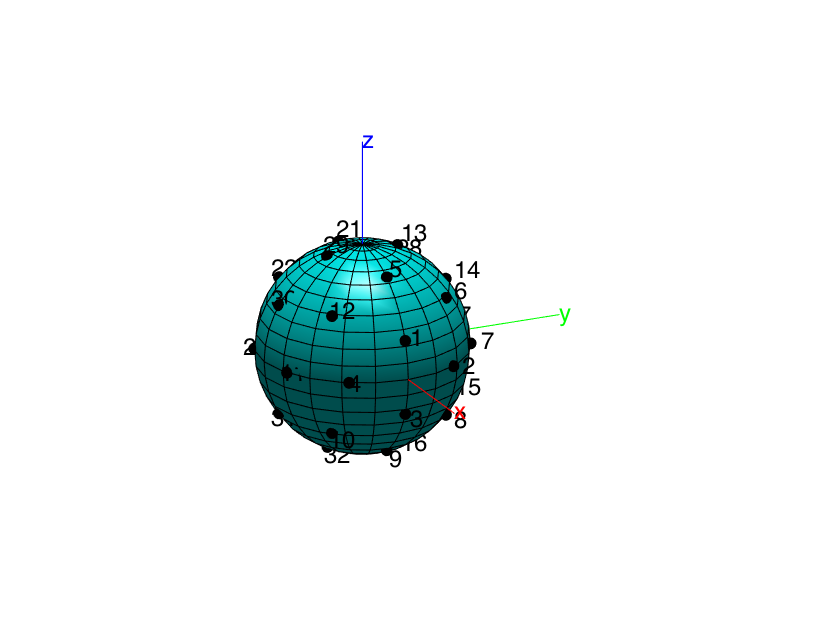
clear all; close all;

% Simulate a nearly uniform array of 32 microphones on a rigid baffle, with
% the specifications of the Eigenmike array [ref2].
mic_dirs_deg = ...
    [0    21;
    32     0;
     0   -21;
   328     0;
     0    58;
    45    35;
    69     0;
    45   -35;
     0   -58;
   315   -35;
   291     0;
   315    35;
    91    69;
    90    32;
    90   -31;
    89   -69;
   180    21;
   212     0;
   180   -21;
   148     0;
   180    58;
   225    35;
   249     0;
   225   -35;
   180   -58;
   135   -35;
   111     0;
   135    35;
   269    69;
   270    32;
   270   -32;
   271   -69];
mic_dirs_rad = mic_dirs_deg*pi/180;
nMics = size(mic_dirs_deg,1);
% Eigenmike radius
R = 0.042;
% Plot microphone array
plotMicArray(mic_dirs_deg, R); view(65,20);
h = gcf; h.Position(3) = 1.5*h.Position(3); h.Position(4) = 1.5*h.Position(4);
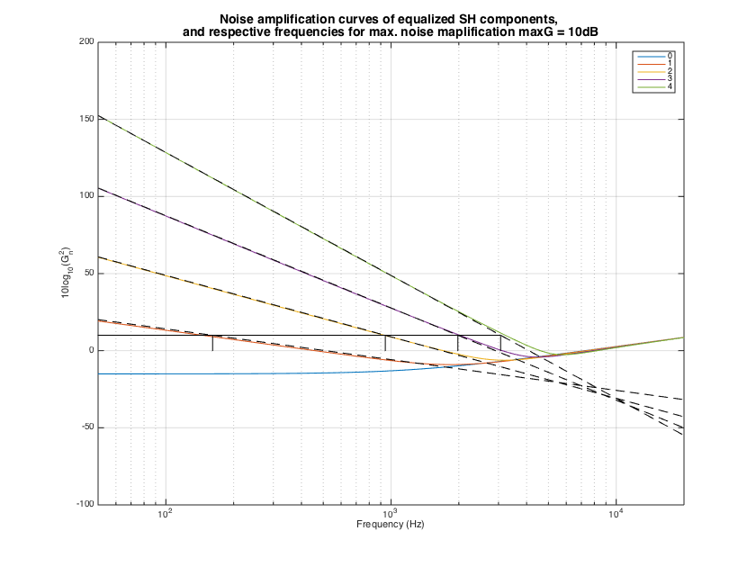
% Type and order of expansion for modeling the array response
arrayType = 'rigid';
c = 343;
f_max = 20000;
kR_max = 2*pi*f_max*R/c;
array_order = ceil(2*kR_max);

% frequency vector
fs = 48000;
Lfilt = 1024;
f = (0:Lfilt/2)'*fs/Lfilt;
kR = 2*pi*f*R/c;
nBins = Lfilt/2+1;

% Do some array analysis of noise and spatial aliasing
sht_order = floor(sqrt(nMics)-1); % approximate for uniformly arranged mics
[ampf, ampf_lin] = sphArrayNoise(R, nMics, sht_order, arrayType, f);
% plot noise power responses
figure
semilogx(f, 10*log10(abs(ampf)));
hold on, semilogx(f, 10*log10(abs(ampf_lin)),'--k')
grid, xlabel('Frequency (Hz)'), ylabel('10log_{10}(G_n^2)'), set(gca, 'xlim', [50 20000])
legend(num2str((0:sht_order)'))
% find limiting frequencies for the specified threshold
maxG_db = 10;
f_lim = sphArrayNoiseThreshold(R, nMics, maxG_db, sht_order, arrayType);
% plot frequencies
semilogx([f(2) f_lim(end)]', ones(2,1)*maxG_db, 'color','k')
for n=1:sht_order
    semilogx([f_lim(n) f_lim(n)], [0 maxG_db], 'k')
end
ht = title(['Noise amplification curves of equalized SH components, ' char(10) 'and respective frequencies for max. noise maplification maxG = ' num2str(maxG_db) 'dB']);
ht.FontSize = 14; h = gcf; h.Position(3) = 1.5*h.Position(3); h.Position(4) = 1.5*h.Position(4);
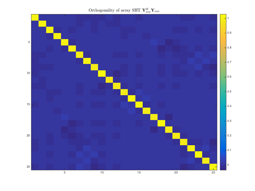
% get spatial aliasing estimates, by SHT order, number of microphone or condition number
f_alias = sphArrayAliasLim(R, nMics, sht_order, mic_dirs_rad);
% plot orthogonality matrix of the microphone arrangement
aziElev2aziPolar = @(dirs) [dirs(:,1) pi/2-dirs(:,2)]; % function to convert from azimuth-inclination to azimuth-elevation
Y_mics = sqrt(4*pi) * getSH(sht_order, aziElev2aziPolar(mic_dirs_rad), 'real'); % real SH matrix for microphones
YY_mics = (1/nMics)*(Y_mics'*Y_mics);
figure
imagesc(YY_mics), colorbar
ht = title( 'Orthogonality of array SHT $\mathbf{Y}_{mic}^H \mathbf{Y}_{mic}$','Interpreter','latex');
ht.FontSize = 14; h = gcf; h.Position(3) = 1.5*h.Position(3); h.Position(4) = 1.5*h.Position(4);
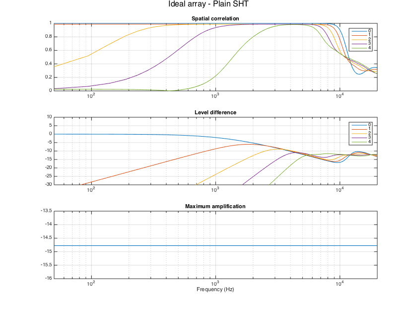
% Obtain responses for a dense grid of directions
[grid_azi, grid_elev] = meshgrid(-180:5:180, -85:5:85);
grid_dirs_deg = [grid_azi(:) grid_elev(:)];
grid_dirs_rad = grid_dirs_deg*pi/180;
[~, H_array_sim] = simulateSphArray(Lfilt, mic_dirs_rad, grid_dirs_rad, arrayType, R, array_order, fs);

% Define an inline function for super-titles in subplots
supertitle = @(title_string) annotation('textbox', [0 0.9 1 0.1],'String', title_string,'EdgeColor', 'none','HorizontalAlignment', 'center','FontSize', 16);

% Apply a plain SHT on the microphone responses without equalization.
M_mic2sh_sht = (1/nMics)*Y_mics';

Y_grid = sqrt(4*pi) * getSH(sht_order, aziElev2aziPolar(grid_dirs_rad), 'real'); % SH matrix for grid directions
%w_grid = getVoronoiWeights(grid_dirs_rad); % get approximate integration weights for grid points
%evaluateSHTfilters(repmat(M_mic2sh_sht, [1 1 nBins]), H_array_sim, fs, Y_grid, w_grid);
evaluateSHTfilters(repmat(M_mic2sh_sht, [1 1 nBins]), H_array_sim, fs, Y_grid);
supertitle('Ideal array - Plain SHT'); h = gcf; h.Position(3) = 1.5*h.Position(3); h.Position(4) = 1.5*h.Position(4);
% Apply single channel regularized inversion, as found e.g. in [ref1]
maxG_dB = 15; % maximum allowed amplification
H_filt = arraySHTfiltersTheory_radInverse(R, nMics, sht_order, Lfilt, fs, maxG_dB);
% combine the per-order filters with the SHT matrix for evaluation of full filter matrix
for kk=1:nBins
    M_mic2sh_radinv(:,:,kk) = diag(replicatePerOrder(H_filt(kk,:),2))*M_mic2sh_sht;
end
evaluateSHTfilters(M_mic2sh_radinv, H_array_sim, fs, Y_grid);
supertitle('Ideal array - Regularized inversion of radial response');
h = gcf; h.Position(3) = 1.5*h.Position(3); h.Position(4) = 1.5*h.Position(4);
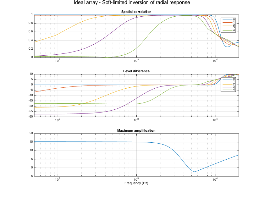
% Apply single channel inversion with soft-limiting, as proposed in [ref3]
H_filt = arraySHTfiltersTheory_softLim(R, nMics, sht_order, Lfilt, fs, maxG_dB);
% combine the per-order filters with the SHT matrix for evaluation of full filter matrix
for kk=1:nBins
    M_mic2sh_softlim(:,:,kk) = diag(replicatePerOrder(H_filt(kk,:),2))*M_mic2sh_sht;
end
evaluateSHTfilters(M_mic2sh_softlim, H_array_sim, fs, Y_grid);
supertitle('Ideal array - Soft-limited inversion of radial response');
h = gcf; h.Position(3) = 1.5*h.Position(3); h.Position(4) = 1.5*h.Position(4);
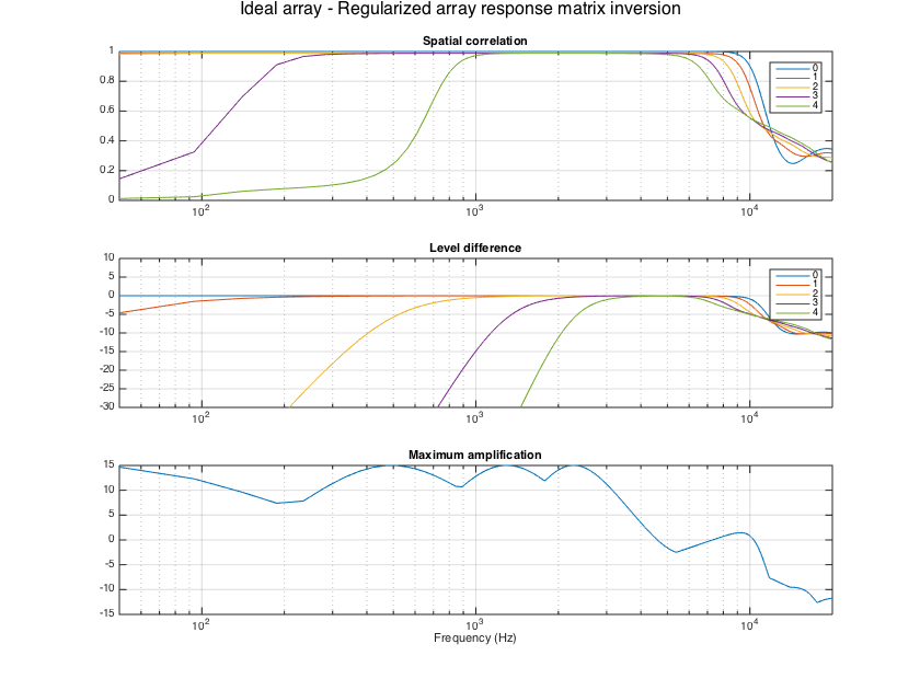
% Invert the full theoretical array response matrix, as proposed in [ref4]
M_mic2sh_regLS = arraySHTfiltersTheory_regLS(R, mic_dirs_rad, sht_order, Lfilt, fs, maxG_dB);
evaluateSHTfilters(M_mic2sh_regLS, H_array_sim, fs, Y_grid);
supertitle('Ideal array - Regularized array response matrix inversion');
h = gcf; h.Position(3) = 1.5*h.Position(3); h.Position(4) = 1.5*h.Position(4);
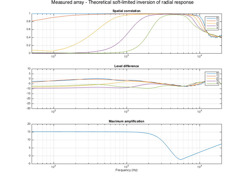
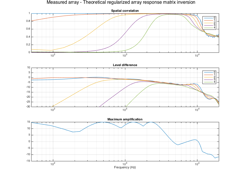
---Measurement based-filters
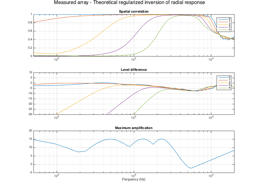
When calibration measurements of the array response exist, it is advantageous to create the filters based on them, to take into account any deviations of the actual array from the theoretical model. In the example below measured responses of an Egenmike array are used, and the filters are evaluated with respect to that.
load('Eigenmike_IRs.mat', 'fs', 'h_mics', 'measurement_dirs_aziElev', 'measurement_area_weights');
grid_dirs_rad = measurement_dirs_aziElev; clear measurement_dirs_aziElev
w_grid = measurement_area_weights; clear measurement_area_weights
Y_grid = sqrt(4*pi) * getSH(sht_order, aziElev2aziPolar(grid_dirs_rad), 'real'); % SH matrix for grid directions
nGrid = length(w_grid);
H_array_meas = fft(h_mics,Lfilt);
H_array_meas = H_array_meas(1:nBins,:,:);

% normalize measured responses close to unity using the mean of responses
% (equivalent to the diffuse omni power)
for kk=1:nBins
    H_kk = squeeze(H_array_meas(kk,:,:));
    tempH = (1/nMics)*sum(H_kk,1).';
    H_mean(kk) = sqrt( real((tempH.*w_grid)'*tempH) );
end
% normalize responses
norm_diff = max(H_mean);
H_array_meas = H_array_meas/norm_diff;

% first show results when applying the theory-devised filters to the
% real Eigenmike array
evaluateSHTfilters(M_mic2sh_radinv, H_array_meas, fs, Y_grid, w_grid);
supertitle('Measured array - Theoretical regularized inversion of radial response');
h = gcf; h.Position(3) = 1.5*h.Position(3); h.Position(4) = 1.5*h.Position(4);
evaluateSHTfilters(M_mic2sh_softlim, H_array_meas, fs, Y_grid, w_grid);
supertitle('Measured array - Theoretical soft-limited inversion of radial response');
h = gcf; h.Position(3) = 1.5*h.Position(3); h.Position(4) = 1.5*h.Position(4);
evaluateSHTfilters(M_mic2sh_regLS, H_array_meas, fs, Y_grid, w_grid);
supertitle('Measured array - Theoretical regularized array response matrix inversion');
h = gcf; h.Position(3) = 1.5*h.Position(3); h.Position(4) = 1.5*h.Position(4);
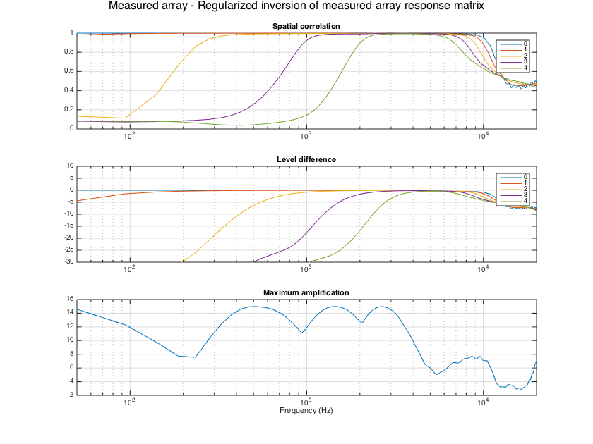
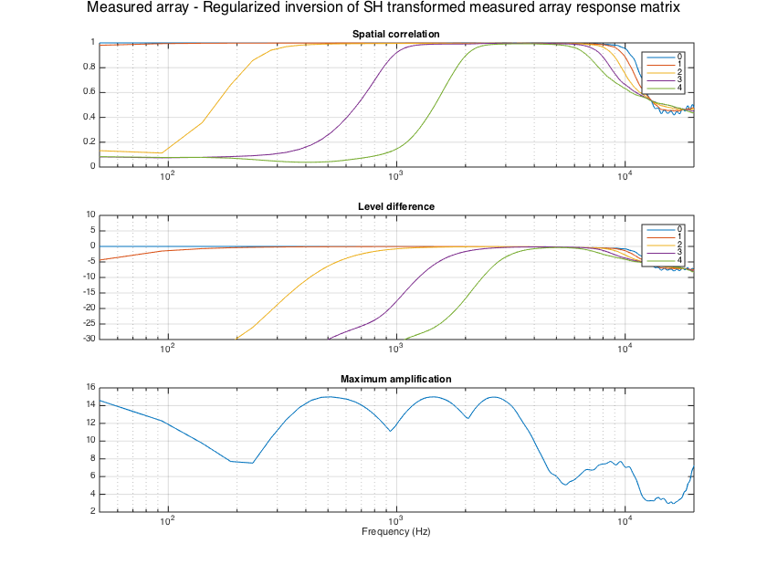
% Compute measurement-based filters and show results
% Invert the measured array response matrix, as proposed in [ref1]
E_mic2sh_regLS = arraySHTfiltersMeas_regLS(H_array_meas, sht_order, grid_dirs_rad, w_grid, Lfilt, maxG_dB);
evaluateSHTfilters(E_mic2sh_regLS, H_array_meas, fs, Y_grid, w_grid);
supertitle('Measured array - Regularized inversion of measured array response matrix');
h = gcf; h.Position(3) = 1.5*h.Position(3); h.Position(4) = 1.5*h.Position(4);

% Invert the SH coefficients of the array response matrix, as proposed in [ref4]
E_mic2sh_regLSHD = arraySHTfiltersMeas_regLSHD(H_array_meas, sht_order, grid_dirs_rad, w_grid, Lfilt, maxG_dB);
evaluateSHTfilters(E_mic2sh_regLSHD, H_array_meas, fs, Y_grid, w_grid);
supertitle('Measured array - Regularized inversion of SH transformed measured array response matrix');
h = gcf; h.Position(3) = 1.5*h.Position(3); h.Position(4) = 1.5*h.Position(4);
SIGNAL-INDEPENDENT BEAMFORMING IN THE SPHERICAL HARMONIC DOMAIN
After the SH signals have been obtained, it is possible to perform beamforming on the SHD. In the frequency band that the SH signals are close to the ideal ones, beamforming is frequency-independent and it corresponds to a weight-and-sum operation of the SH signals. The beamforming weights can be derived analytically for various common beampatterns and for the available order of the SH signals. Beampatterns maintain their directivity for all directions in the SHD, and if they are axisymmetric their rotation to an arbitrary direction becomes very simple.
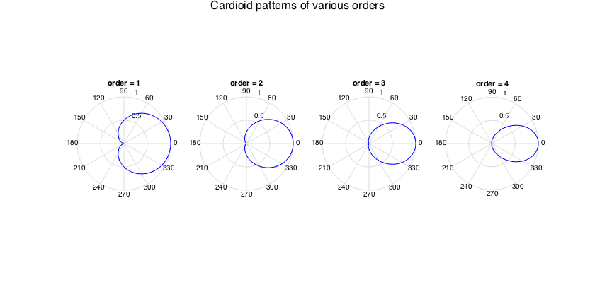
The following axisymmetric patterns are included in the library:
- cardioid [single null at opposite of the look-direction]
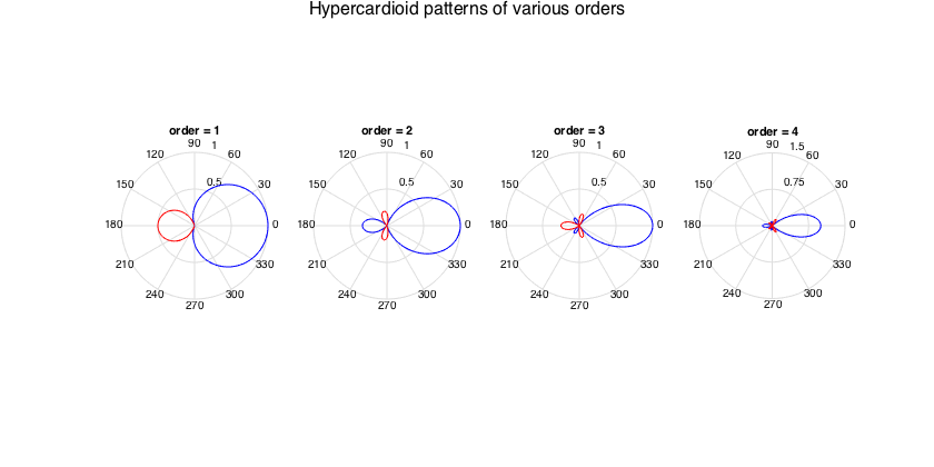
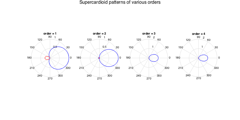
- supercardioid (up to 4th-order) [ref5] [maximum front-to-back rejection ratio]
- hypercardioid/superdirective/regular/plane-wave decomposition beamformer [maximum directivity factor]
- max-energy vector (almost super-cardioid) [ref6] [maximum intensity vector under isotropic diffuse conditions]
- Dolph-Chebyshev [ref7] [sidelobe level control]
- arbitrary patterns of differential form [ref8] [weighted cosine power series]
- patterns corresponding to real- and symmetrically-weighted linear array [ref9]
and some non-axisymmetric cases:
- closest beamformer to a given directional function [best least-squares approximation]
- acoustic velocity beamformers for a given spatial filter [ref10] [capture the acoustic velocity of a directionally-weighted soundfield]
The following code examples illustrate most of these patterns.
clear all; close all;
% Define an inline function for super-titles in subplots
supertitle = @(title_string) annotation('textbox', [0 0.9 1 0.1],'String', title_string,'EdgeColor', 'none','HorizontalAlignment', 'center','FontSize', 16);
---Cardioids
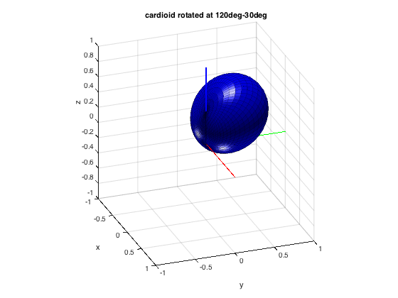
% get beamforming weights for orders 1-4 and plot pattern
figure
for n=1:4
    h = subplot(1,4,n);
    w_n = beamWeightsCardioid2Spherical(n);
    plotAxisymPatternFromCoeffs(w_n, h)
    title(['order = ' num2str(n)])
end
supertitle('Cardioid patterns of various orders');
h = gcf; h.Position(3) = 1.5*h.Position(3);
% get the beamforming weights for a rotated 3rd-order cardioid to 120deg azi
% and 60deg elevation
w_n = beamWeightsCardioid2Spherical(3);
azi = 2*pi/3;
incl = pi/2-pi/6; % inclination instead of elevation is used in this function
w_nm = rotateAxisCoeffs(w_n, incl, azi, 'real');
plotSphFunctionCoeffs(w_nm, 'real', 5, 5, 'real'), axis([-1 1 -1 1 -1 1]), view(70,25); title('cardioid rotated at 120deg-30deg')
---Hypercardioids (regular spherical beamformer, plane-wave decomposition, superdirective, or max-DI)
% get beamforming weights for orders 1-4 and plot pattern
figure
for n=1:4
    h = subplot(1,4,n);
    w_n = beamWeightsHypercardioid2Spherical(n);
    plotAxisymPatternFromCoeffs(w_n, h)
    title(['order = ' num2str(n)])
end
supertitle('Hypercardioid patterns of various orders');
h = gcf; h.Position(3) = 1.5*h.Position(3);
---Supercardioids (max front-to-back power ratio)
Note that the coefficients for these are hard-coded and defined up to order 4. The coefficients have been converted from differential array coefficients found in [ref]. An analytical formula for supercardioids of any order directly in the SHD is not known to the author.
% get beamforming weights for orders 1-4 and plot pattern
figure
for n=1:4
    h = subplot(1,4,n);
    w_n = beamWeightsSupercardioid2Spherical(n);
    plotAxisymPatternFromCoeffs(w_n, h)
    title(['order = ' num2str(n)])
end
supertitle('Supercardioid patterns of various orders');
h = gcf; h.Position(3) = 1.5*h.Position(3);
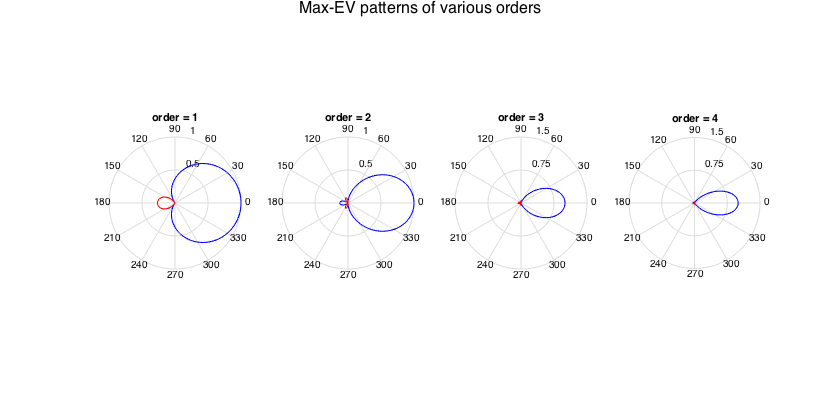
---Max-EV (energy vector) patterns
These patterns originate from literature on Ambisonics [ref]. They do not optimize any of the standard array processing metrics. Instead they maximize the length of the resulting vector, if a unit vector is weighted with the squared pattern and integrated over all directions. From an acoustic standpoint, this could be the pattern that maximizes the acoustic intensity vector in an isotropic diffuse field. They are relevant in the design of panning functions. In practice they are very similar (but not equal) to supercardioids, and they can easily be generated analytically for any order.
% get beamforming weights for orders 1-4 and plot pattern
figure
for n=1:4
    h = subplot(1,4,n);
    w_n = beamWeightsMaxEV(n);
    plotAxisymPatternFromCoeffs(w_n, h)
    title(['order = ' num2str(n)])
end
supertitle('Max-EV patterns of various orders');
h = gcf; h.Position(3) = 1.5*h.Position(3);
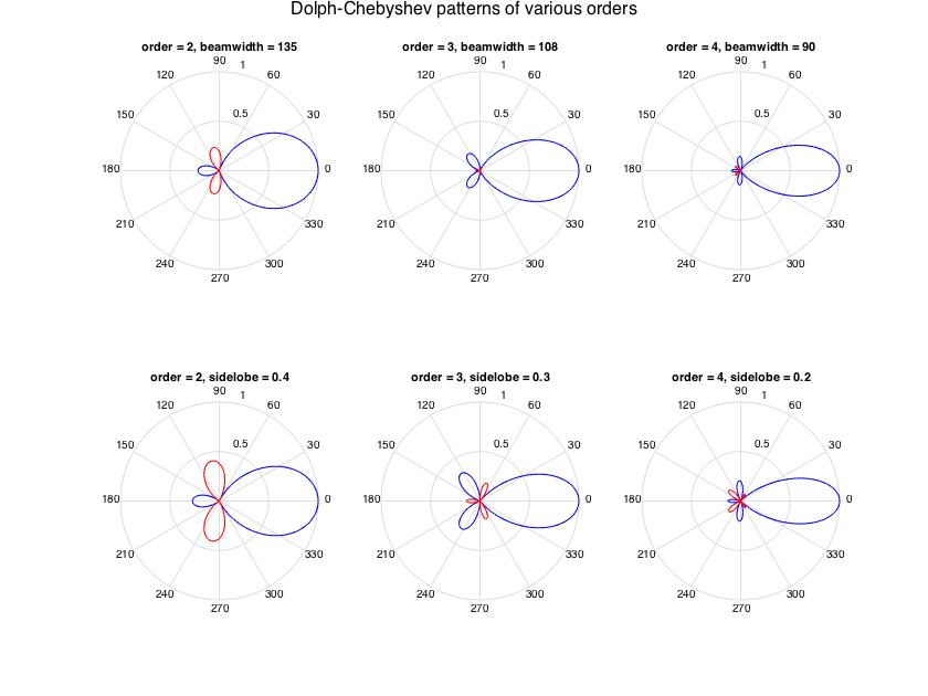
---Dolph-Chebyshev beampatterns
Here the pattern is determined, apart from the order, from a specification of the sidelobe level, or the null-to-null mainlobe width. The generating formula is as found in [ref7].
% get beamforming weights for orders 2-4 and plot pattern
figure
bwidths = [3*pi/4; 3*pi/5; pi/2]; % beamwidths for plotting
slobes = [0.4, 0.3, 0.2]; % sidelobe leves for plotting
for n=2:4
    h = subplot(2,3,n-1);
    w_n = beamWeightsDolphChebyshev2Spherical(n, 'width', bwidths(n-1));
    plotAxisymPatternFromCoeffs(w_n, h)
    title(['order = ' num2str(n) ', beamwidth = ' num2str(rad2deg(bwidths(n-1)))])
end
for n=2:4
    h = subplot(2,3,3+(n-1));
    w_n = beamWeightsDolphChebyshev2Spherical(n, 'sidelobe', slobes(n-1));
    plotAxisymPatternFromCoeffs(w_n, h)
    title(['order = ' num2str(n) ', sidelobe = ' num2str(slobes(n-1))])
end
supertitle('Dolph-Chebyshev patterns of various orders');
h = gcf; h.Position(3) = 1.5*h.Position(3); h.Position(4) = 1.5*h.Position(4);
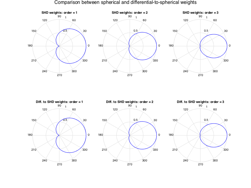
---Differential arrays
Differential arrays of N+1 microphones can generate any axisymmetric pattern 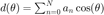 of order N, with differential weights a_n. The following function transforms the differential weights to SH weights suitable for spherical processing, with the transformation done as in [ref8]. This is useful for obtaining weights for patterns that are defined using the differential form, see e.g. [ref5].
% Generate cardioid beamformers directly in the SHD, and compare with
% cardioids defined as differential weights first, and then transformed to
% spherical.
figure
for n=1:3
    h = subplot(2,3,n);
    w_n = beamWeightsCardioid2Spherical(n);
    plotAxisymPatternFromCoeffs(w_n, h)
    title(['SHD weights: order = ' num2str(n)])
    h = subplot(2,3,3+n);
    a_n = beamWeightsCardioid2Differential(n); % generate weights for cardioids using the differential form
    b_n = beamWeightsDifferential2Spherical(a_n); % convert from differential to spherical
    plotAxisymPatternFromCoeffs(b_n, h)
    title(['Diff. to SHD weights: order = ' num2str(n)])
end
supertitle('Comparison between spherical and differential-to-spherical weights');
h = gcf; h.Position(3) = 1.5*h.Position(3); h.Position(4) = 1.5*h.Position(4);
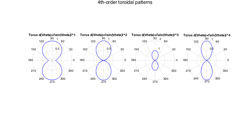
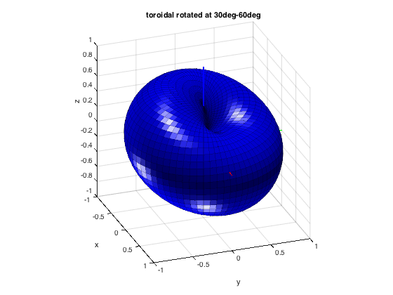
---Arbitrary beampatterns
It is possible to obtain spherical beamforming weights for an arbitrary beamforming pattern, as a best least-squares approximation to it for a certain order. This can be done by performing a discrete SHT on the target pattern. The example below obtains the weights for axisymmetric toroidal patterns.
figure
for n=1:4
    h = subplot(1,4,n);

    % Define a function describing the target pattern: toroidal pattern raised
    % to the n-th power
    fPattern = @(azi,elev) ones(size(azi)).*abs(cos(elev)).^n;
    % Get beamforming weights for order 4 patterns
    order = 4;
    w_nm = beamWeightsFromFunction(fPattern, order);
    % keep only the m=0 weights, due to axisymmetry
    w_n = extractAxisCoeffs(w_nm);
    plotAxisymPatternFromCoeffs(w_n, h)
    title(['Torus d(\theta)=|\sin(\theta)|^' num2str(n)])
end
supertitle('4th-order toroidal patterns');
h = gcf; h.Position(3) = 1.5*h.Position(3);
% rotate a toroidal pattern to 30deg azi and 60deg elevation
fPattern = @(azi,elev) ones(size(azi)).*abs(cos(elev));
w_n = extractAxisCoeffs(beamWeightsFromFunction(fPattern, order));
azi = pi/6;
elev = pi/3;
w_nm = rotateAxisCoeffs(w_n, pi/2-elev, azi, 'real'); % inclination instead of elevation is used in this function
plotSphFunctionCoeffs(w_nm, 'real', 5, 5, 'real'), axis([-1 1 -1 1 -1 1]), view(70,25); title('toroidal rotated at 30deg-60deg')
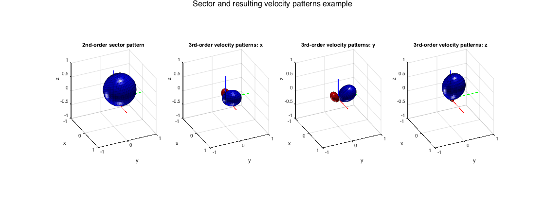
---Weighted velocity beamformers
A continuous amplitude distribution of plane waves incident from all directions results in a certain acoustic pressure and velocity at the origin. The pressure corresponds to omnidirectional pickup, while the components of the velocity vector can be captured by three dipole patterns oriented along the Certesian axis. If the sound-field distribution has been weighted by some directional pattern, e.g. some beamformer, then the resulting velocity components can be captured by specific patterns, products of the beamformer and the dipoles, as shown in [ref10]. These velocity beamformers have some applications to estimation of acoustic velocity or intensity at directionally constrained regions. Note that the velocity weights are one order greater than the beamfomrer that generates them.
% Define a 2nd-order cardioid as the directional weighting, oriented at
% 30deg azi and 60deg elevation.
order_sec = 2;
w_n = beamWeightsCardioid2Spherical(order_sec); % sector order cardioid
A_xyz = computeVelCoeffsMtx(order_sec); % compute transformation matrices for velocity patterns
v_nm = beamWeightsVelocityPatterns(w_n, [azi elev], A_xyz, 'real'); % compute velocity weights for rotated cardioid
% plot sector and velocity patterns
figure
h_ax = subplot(141);
plotSphFunctionCoeffs(rotateAxisCoeffs(w_n,pi/2-elev,azi,'real'), 'real', 5, 5, 'real', h_ax)
title('2nd-order sector pattern'), view(65,30), axis([-1 1 -1 1 -1 1])
vel_labels = {'x','y','z'};
for n=1:3
    h_ax = subplot(1,4,n+1);
    plotSphFunctionCoeffs(v_nm(:,n), 'real', 5, 5, 'real', h_ax)
    title(['3rd-order velocity patterns: ' vel_labels{n}]), view(65,30), axis([-1 1 -1 1 -1 1])
end
supertitle('Sector and resulting velocity patterns example')
h = gcf; h.Position(3) = 2*h.Position(3);
SIGNAL-DEPENDENT AND PARAMETRIC BEAMFORMING
Contrary to the fixed beamformers of the previous section, parametric and signal-dependent beamformers use information about the signals of interest, given either in terms of acoustical parameters, such as DoAs of the sources, or extracted through the second-order statistics of the array signals given through their spatial covariance matrix (or a combination of the two)
% The following examples are included in the library:
%
% * plane-wave decomposition (PWD) beamformer at desired DoA, with
% nulls at other specified DoAs
% * null-steering beamformer at specified DoAs with constraint on
% omnidirectional response otherwise
% * minimum-variance distortioneless response (MVDR) in the SHD
% * linearly-constrained minimum variance (LCMV) beamformer in the SHD
% * informed parametric multi-wave multi-channel Wiener spatial filter
% (iPMMW) in the SHD [ref]
%
% The following code examples illustrates these methods.

clear all; close all;
% Define an inline function for super-titles in subplots
supertitle = @(title_string) annotation('textbox', [0 0.9 1 0.1],'String', title_string,'EdgeColor', 'none','HorizontalAlignment', 'center','FontSize', 16);
% function to convert from azimuth-inclination to azimuth-elevation
aziElev2aziPolar = @(dirs) [dirs(:,1) pi/2-dirs(:,2)];
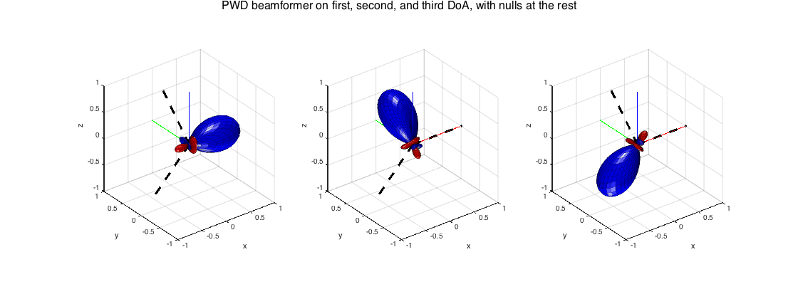
---Plane-wave decomposition beamformer with null-steering
This simple beamformer produces the beamforming weight vectors for a number of specified directions, where each vector corresponds to a PWD beamformer at the specific direction, with nulls at the rest.
% signal modeling
order = 3;
src_dirs = [0 0; pi/2 pi/4; pi -pi/4];
src_xyz = unitSph2cart(src_dirs);
% compute beamformer weights and plot results
W_nullpwd = sphNullformer_pwd(order, src_dirs);
figure
h_ax = subplot(131); plotSphFunctionCoeffs(W_nullpwd(:,1), 'real', 5, 5, 'real', h_ax); view(3), axis([-1 1 -1 1 -1 1])
line([0 0 0; src_xyz(:,1)'],[0 0 0; src_xyz(:,2)'],[0 0 0; src_xyz(:,3)'],'color','k','linewidth',3,'linestyle','--')
h_ax = subplot(132); plotSphFunctionCoeffs(W_nullpwd(:,2), 'real', 5, 5, 'real', h_ax); view(3), axis([-1 1 -1 1 -1 1])
line([0 0 0; src_xyz(:,1)'],[0 0 0; src_xyz(:,2)'],[0 0 0; src_xyz(:,3)'],'color','k','linewidth',3,'linestyle','--')
h_ax = subplot(133); plotSphFunctionCoeffs(W_nullpwd(:,3), 'real', 5, 5, 'real', h_ax); view(3), axis([-1 1 -1 1 -1 1])
line([0 0 0; src_xyz(:,1)'],[0 0 0; src_xyz(:,2)'],[0 0 0; src_xyz(:,3)'],'color','k','linewidth',3,'linestyle','--')
supertitle('PWD beamformer on first, second, and third DoA, with nulls at the rest');
h = gcf; h.Position(3) = 2*h.Position(3);
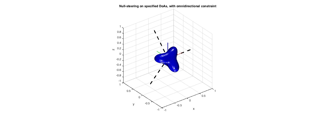
---Nullformer for diffuse sound extraction
This beamformer puts nulls at the directions of the sources, while aiming to preserve as much omnidirectional response as possible. It is similar to [ref11], but in the SHD the diffuse coherence vector simplifies to unity for the omni channel (first SH signal) and zeros for the rest, due to the orthogonality of the SHs.
% signal modeling
order = 3;
src_dirs = [0 0; pi/2 pi/4; pi -pi/4];
src_xyz = unitSph2cart(src_dirs);
% compute beamformer weights and plot results
w_nulldiff = sphNullformer_diff(order, src_dirs);
plotSphFunctionCoeffs(w_nulldiff, 'real', 5, 5, 'real'); view(3), axis([-1 1 -1 1 -1 1])
line([0 0 0; src_xyz(:,1)'],[0 0 0; src_xyz(:,2)'],[0 0 0; src_xyz(:,3)'],'color','k','linewidth',3,'linestyle','--')
title('Null-steering on specified DoAs, with omnidirectional constraint');
h = gcf; h.Position(3) = 2*h.Position(3);
---MVDR
A classic adaptive beamformer. In the example below the source powers and directions are known and the SH covariance matrix is constructed and passed to the MVDR. Multiple sets of weights are computed if multiple directions are passed to the MVDR, one for each distortionless response. The method is exactly the same as the MVDR in the space (sensor) domain, with the array steering vectors replaced by SHs.
% signal modeling
order = 3;
nSH = (order+1)^2;
src_dirs = [0 0; pi/2 0; 0 pi/4];
src_xyz = unitSph2cart(src_dirs);
Y_src = getSH(order, aziElev2aziPolar(src_dirs), 'real');
stVec = Y_src';
P_src = diag([1 1 1]);
P_diff = 1;
sphCOV = stVec*P_src*stVec' + P_diff*eye(nSH)/(4*pi);
% compute beamformer weights and plot results
W_mvdr = sphMVDR(sphCOV, src_dirs);
figure
h_ax = subplot(131); plotSphFunctionCoeffs(W_mvdr(:,1), 'real', 5, 5, 'real', h_ax); view(3), axis([-1 1 -1 1 -1 1])
line([0 0 0; src_xyz(:,1)'],[0 0 0; src_xyz(:,2)'],[0 0 0; src_xyz(:,3)'],'color','k','linewidth',3,'linestyle','--')
h_ax = subplot(132); plotSphFunctionCoeffs(W_mvdr(:,2), 'real', 5, 5, 'real', h_ax); view(3), axis([-1 1 -1 1 -1 1])
line([0 0 0; src_xyz(:,1)'],[0 0 0; src_xyz(:,2)'],[0 0 0; src_xyz(:,3)'],'color','k','linewidth',3,'linestyle','--')
h_ax = subplot(133); plotSphFunctionCoeffs(W_mvdr(:,3), 'real', 5, 5, 'real', h_ax); view(3), axis([-1 1 -1 1 -1 1])
line([0 0 0; src_xyz(:,1)'],[0 0 0; src_xyz(:,2)'],[0 0 0; src_xyz(:,3)'],'color','k','linewidth',3,'linestyle','--')
supertitle('MVDR beamformer on first, second, and third DoA');
h = gcf; h.Position(3) = 2*h.Position(3);

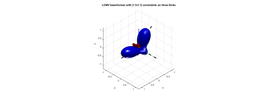
---LCMV
The LCMV, or linearly-constrained minimum variance beamformer is a generalization of the MVDR, where multiple directional constraints can be specified. Th example below constructs and serves directly the SH covariance matrix as in the MVDR example. The method is exactly the same as the LCMV in the space (sensor) domain, with the array steering vectors replaced by SHs.
% signal modeling
order = 3;
nSH = (order+1)^2;
src_dirs = [0 0; pi/2 0; pi pi/4];
src_xyz = unitSph2cart(src_dirs);
Y_src = getSH(order, aziElev2aziPolar(src_dirs), 'real');
stVec = Y_src';
P_src = diag([1 1 1]); % unit powers for the three sources
P_diff = 1; % unit power for the diffuse sound
sphCOV = stVec*P_src*stVec' + P_diff*eye(nSH)/(4*pi);
% compute beamformer weights and plot results
constraints = [1 0.5 1]';
w_lcmv = sphLCMV(sphCOV, src_dirs, constraints);
plotSphFunctionCoeffs(w_lcmv, 'real', 5, 5, 'real'); view(135,35), axis(1.2*[-1 1 -1 1 -1 1])
line([0 0 0; 1.2*src_xyz(:,1)'],[0 0 0; 1.2*src_xyz(:,2)'],[0 0 0; 1.2*src_xyz(:,3)'],'color','k','linewidth',3,'linestyle','--')
title('LCMV beamformer with [1 0.5 1] constraints on three DoAs');
h = gcf; h.Position(3) = 2*h.Position(3);
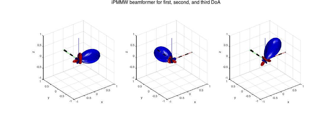
---iPMMW
The iPMMW, as has been proposed in [ref12], is an optimal beamformer for extraction of multiple plane-wave sounds, with a trade-off between signal distortion and diffuse and spatially-white noise suppression. It combines an LCMV beamformer with a Multi-channel Wiener filter. It relies on estimation of sensor noise power, diffuse signal power, source signal powers, and their DoAs. In the example below we assume that the respective quantities have been estimated perfectly and they are served to the beamformer.
% SIGNAL MODELING
order = 3;
nSH = (order+1)^2;
src_dirs = [0 0; pi/2 0; pi pi/4];
src_xyz = unitSph2cart(src_dirs);
Y_src = getSH(order, aziElev2aziPolar(src_dirs), 'real');
stVec = Y_src';
% source powers
P_src = [1 2 0.7];
% diffuse power at -10dB
P_diff = 0.1;
% noise power at SH signals at -30dB
P_noise = 0.001;
% SIGNAL STATISTICS
% signal covariance matrix (assuming uncorrelated sources)
Ss = stVec*diag(P_src)*stVec';
% diffuse field coherence matrix in the SHD (identity due to orthogonality)
Gamma_d = eye(nSH)/(4*pi);
% diffuse sound covariance matrix
Sd = P_diff*Gamma_d;
% Noise covariance matrix. Identity for simplicity now. Commonly this is
% an identity matrix for sensor noise modeling only. For a more realistic
% SH noise, the transformation of the microphone signals and the equalization
% has to be taken into account. In general this is still diagonal below aliasing,
% but not white.
Sn = P_noise*eye(nSH);
% SH signal statistics
sphCOV = Ss + Sd + Sn;

% compute beamformer weights and plot results
[W_pmmw, Pd_est, Ps_est] = sphiPMMW(sphCOV, Sn, src_dirs);
figure
h_ax = subplot(131); plotSphFunctionCoeffs(W_mvdr(:,1), 'real', 5, 5, 'real', h_ax); view(3), axis([-1 1 -1 1 -1 1])
line([0 0 0; src_xyz(:,1)'],[0 0 0; src_xyz(:,2)'],[0 0 0; src_xyz(:,3)'],'color','k','linewidth',3,'linestyle','--')
h_ax = subplot(132); plotSphFunctionCoeffs(W_mvdr(:,2), 'real', 5, 5, 'real', h_ax); view(3), axis([-1 1 -1 1 -1 1])
line([0 0 0; src_xyz(:,1)'],[0 0 0; src_xyz(:,2)'],[0 0 0; src_xyz(:,3)'],'color','k','linewidth',3,'linestyle','--')
h_ax = subplot(133); plotSphFunctionCoeffs(W_mvdr(:,3), 'real', 5, 5, 'real', h_ax); view(3), axis([-1 1 -1 1 -1 1])
line([0 0 0; src_xyz(:,1)'],[0 0 0; src_xyz(:,2)'],[0 0 0; src_xyz(:,3)'],'color','k','linewidth',3,'linestyle','--')
supertitle('iPMMW beamformer for first, second, and third DoA');
h = gcf; h.Position(3) = 2*h.Position(3);
DIRECTION-OF-ARRIVAL (DoA) ESTIMATION IN THE SHD
Direction of arrival (DoA) estimation can be done by a steered-response power approach, steering a beamformer on a grid and checking for peaks on the power output, or by a subspace approach such as MUSIC. Another alternative is to utilize the acoustic intensity vector, obtained from the first-order signals, which its temporal and spatial statistics reveal information about presence and distribution of sound sources.
A few examples of DoA estimation in the SHD are included in the library:
- Steered-response power DoA estimation, based on plane-wave decomposition (regular) beamforming
- Steered-response power DoA estimation, based on MVDR beamforming
- Acoustic intensity vector DoA estimation
- Eigenbeam-MUSIC DoA estimation
The following code examples illustrates use of these methods.
aziElev2aziPolar = @(dirs) [dirs(:,1) pi/2-dirs(:,2)]; % function to convert from azimuth-inclination to azimuth-elevation
grid_dirs = grid2dirs(5,5,0,0); % Grid of directions to evaluate DoA estimation
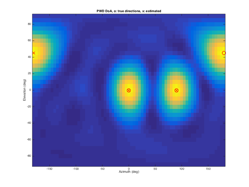
---Plane-wave decomposition power map
This is the simplest approach, in which a (regular) plane-wave decomposition beamformer is steered to multiple directions on a grid, forming a power map. Peak finding then on the map determines potential source DoAs. The spatial resolution of this approach is limited by the available order of the SH signals, and for low orders is also low.
% signal modeling
order = 3;
nSH = (order+1)^2;
src_dirs = [0 0; pi/2 0; pi pi/4];
nSrc = size(src_dirs,1);
Y_src = getSH(order, aziElev2aziPolar(src_dirs), 'real');
stVec = Y_src';
P_src = diag([1 1 1]); % unit powers for the three sources
P_diff = 1; % unit power for the diffuse sound
sphCOV = stVec*P_src*stVec' + P_diff*eye(nSH)/(4*pi);
% DoA estimation
[P_pwd, est_dirs_pwd] = sphPWDmap(sphCOV, grid_dirs, nSrc);
est_dirs_pwd = est_dirs_pwd*180/pi;
% plots results
plotDirectionalMapFromGrid(P_pwd, 5, 5, [], 0, 0);
src_dirs_deg = src_dirs*180/pi;
line_args = {'linestyle','none','marker','o','color','r', 'linewidth',1.5,'markersize',12};
line(src_dirs_deg(:,1), src_dirs_deg(:,2), line_args{:});
line_args = {'linestyle','none','marker','x','color','r', 'linewidth',1.5,'markersize',12};
line(est_dirs_pwd(:,1), est_dirs_pwd(:,2), line_args{:});
xlabel('Azimuth (deg)'), ylabel('Elevation (deg)'), title('PWD DoA, o: true directions, x: estimated')
h = gcf; h.Position(3) = 1.5*h.Position(3); h.Position(4) = 1.5*h.Position(4);
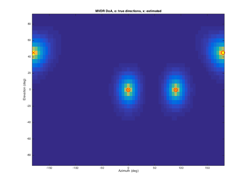
---MVDR power map
This is similar to the PWD estimation, but the power map is formed with a MVDR beamformer. Since statistics of the signals are taken into account in this case, the spatial resolution can be significantly higher. However, due to an incoherence assumption on the source signals, MVDR estimates can be biased by presence of coherent source (e.g. reflections).
% signal modeling
order = 3;
nSH = (order+1)^2;
src_dirs = [0 0; pi/2 0; pi pi/4];
nSrc = size(src_dirs,1);
Y_src = getSH(order, aziElev2aziPolar(src_dirs), 'real');
stVec = Y_src';
P_src = diag([1 1 1]); % unit powers for the three sources
P_diff = 1; % unit power for the diffuse sound
sphCOV = stVec*P_src*stVec' + P_diff*eye(nSH)/(4*pi);
% DoA estimation
[P_mvdr, est_dirs_mvdr] = sphMVDRmap(sphCOV, grid_dirs, nSrc);
est_dirs_mvdr = est_dirs_mvdr*180/pi;
% plots results
plotDirectionalMapFromGrid(P_mvdr, 5, 5, [], 0, 0);
src_dirs_deg = src_dirs*180/pi;
line_args = {'linestyle','none','marker','o','color','r', 'linewidth',1.5,'markersize',12};
line(src_dirs_deg(:,1), src_dirs_deg(:,2), line_args{:});
line_args = {'linestyle','none','marker','x','color','r', 'linewidth',1.5,'markersize',12};
line(est_dirs_mvdr(:,1), est_dirs_mvdr(:,2), line_args{:});
xlabel('Azimuth (deg)'), ylabel('Elevation (deg)'), title('MVDR DoA, o: true directions, x: estimated')
h = gcf; h.Position(3) = 1.5*h.Position(3); h.Position(4) = 1.5*h.Position(4);
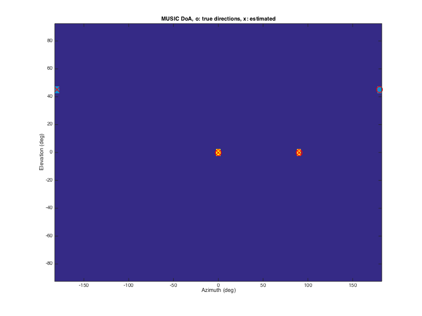
---MUSIC spectrum
The MUSIC method decomposes the spatial correlation matrix of the Sh signals into a signal dominated-subspace, and a noise-dmoniated subspace. Assuming orthogonality between the two, the MUSIC spectrum gives in a very fine resolution view of source DoAs in the sound-field. However that assumption can be violated again in the presence of correlated sources (e.g. early relfections), in which case additional processing should be employed to decorrelate these components.
% signal modeling
order = 3;
nSH = (order+1)^2;
src_dirs = [0 0; pi/2 0; pi pi/4];
nSrc = 3;
Y_src = getSH(order, aziElev2aziPolar(src_dirs), 'real');
stVec = Y_src';
P_src = diag([1 1 1]); % unit powers for the three sources
P_diff = 1; % unit power for the diffuse sound
sphCOV = stVec*P_src*stVec' + P_diff*eye(nSH)/(4*pi);
% DoA estimation
[P_music, est_dirs_music] = sphMUSIC(sphCOV, grid_dirs, nSrc);
est_dirs_music = est_dirs_music*180/pi;
% plots results
plotDirectionalMapFromGrid(P_music, 5, 5, [], 0, 0);
src_dirs_deg = src_dirs*180/pi;
line_args = {'linestyle','none','marker','o','color','r', 'linewidth',1.5,'markersize',12};
line(src_dirs_deg(:,1), src_dirs_deg(:,2), line_args{:});
line_args = {'linestyle','none','marker','x','color','r', 'linewidth',1.5,'markersize',12};
line(est_dirs_music(:,1), est_dirs_music(:,2), line_args{:});
xlabel('Azimuth (deg)'), ylabel('Elevation (deg)'), title('MUSIC DoA, o: true directions, x: estimated')
h = gcf; h.Position(3) = 1.5*h.Position(3); h.Position(4) = 1.5*h.Position(4);
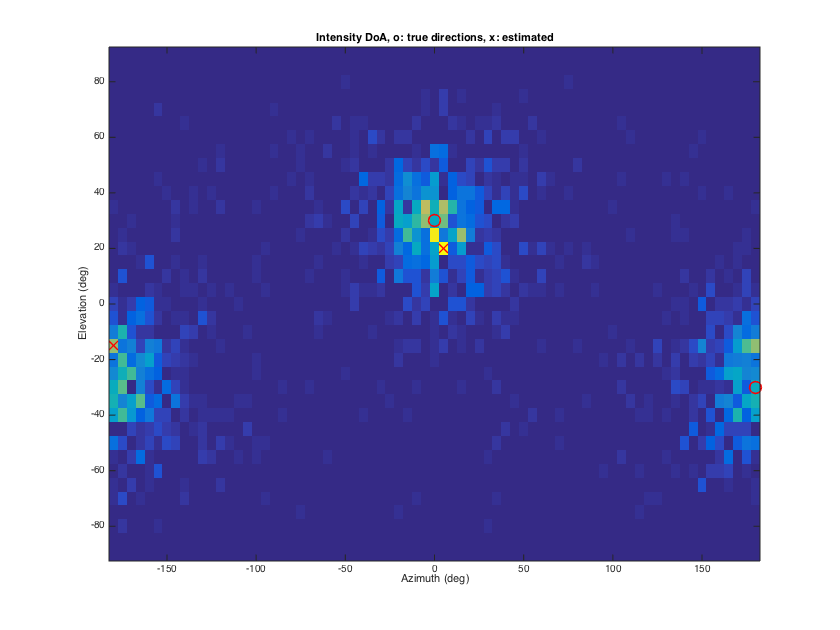
---Intensity vector DoA estimation
The acoustic intensity vector points to the opposite of the source DoA, for a single source, and its time average does the same in presence of a single source and uncorrelated diffuse sound. In presence of multiple active sources, the intensity DoA estimates fluctuate between and around the true DoAs. In this case intensity histograms, and subsequent fitting of distributions can be used to give multiple DoA estimates.
% Source signal modeling
% three unit power white noise sources
lSig = 100000; % samples
src_dirs = [0 pi/6; pi -pi/6];
nSrc = size(src_dirs,1);
srcsig = randn(nSrc, lSig);
order = 1;
nSH = (order+1)^2;
Y_src = getSH(order, aziElev2aziPolar(src_dirs), 'real');
A_dir = Y_src';
sh_dirsig = A_dir*srcsig; % SH signals for sources
% Diffuse signal modeling
[~, diff_dirs] = getTdesign(21); % get dense uniform distribution of directions
nDiff = size(diff_dirs,1);
Pdiff = 1; % diffuse sound power at 0dB
diffsig = sqrt(Pdiff/nDiff)*randn(nDiff, lSig);
Y_diff = getSH(order, aziElev2aziPolar(diff_dirs), 'real');
A_diff = Y_diff';
sh_diffsig = A_diff*diffsig; % SH signals for diffuse sound
% SH signals
shsig = sh_dirsig+sh_diffsig;

% acoustic intensity estimation
% convert to pressure velocity
M_sh2pv = beamWeightsPressureVelocity('real');
pvsig = M_sh2pv*shsig(1:4,:);
% partition the signal into 100 sample buffers with 50% overlap
lBuf = 100;
lHop = 50;
nBuf = lSig/lHop;
pvsig_buf = zeros(nSH, lBuf, lSig/lHop);
for ns=1:nSH
    pvsig_buf(ns,:,:) = buffer(pvsig(ns,:)', lBuf, lHop);
end
% compute correlations of pressure-velocity for each partition, for
% short-time estimates of intensity vector
Iv = zeros(nBuf,3);
for nb=1:nBuf
    p = pvsig_buf(1,:,nb);
    v = pvsig_buf(2:4,:,nb);
    Iv(nb,:) = sum((ones(3,1)*p) .* v, 2);
end
% DoA estimation
[I_hist, est_dirs_iv] = sphIntensityHist(Iv, grid_dirs, nSrc);
est_dirs_iv = est_dirs_iv*180/pi;
% plots results
plotDirectionalMapFromGrid(I_hist, 5, 5, [], 0, 0);
src_dirs_deg = src_dirs*180/pi;
line_args = {'linestyle','none','marker','o','color','r', 'linewidth',1.5,'markersize',12};
line(src_dirs_deg(:,1), src_dirs_deg(:,2), line_args{:});
line_args = {'linestyle','none','marker','x','color','r', 'linewidth',1.5,'markersize',12};
line(est_dirs_iv(:,1), est_dirs_iv(:,2), line_args{:});
xlabel('Azimuth (deg)'), ylabel('Elevation (deg)'), title('Intensity DoA, o: true directions, x: estimated')
h = gcf; h.Position(3) = 1.5*h.Position(3); h.Position(4) = 1.5*h.Position(4);
DIFFUSENESS AND DIRECT-TO-DIFFUSE RATIO (DDR) ESTIMATION
Diffuseness is a measure of how close a sound-field represents ideal diffuse field conditions, meaning a sound-field of plane waves with random amplitudes and incident from random directions, but with constant mean energy density, or equivalently constant power distribution from all directions (isotropy). There are measures of diffuseness that consider point to point quantities, here however we focus on measures that consider the directional distribution, and relate to the SHD. In the case of a single source of power  and an ideal diffuse field of power
  , diffuseness
  is directly related to the direct-to-diffuse ratio (DDR)
  , with the relation
  . In the case of multiple sources
  , an ideal diffuseness can be defined as
  and DDR as
  . Diffuseness is useful in a number of tasks - for acoustic analysis, for parametric spatial sound rendering of room impulse responses (e.g SIRR) or spatial sound recordings (e.g. DirAC), or for constructing filters for diffuse sound suppresion.
The following diffuseness measures are implemented
- intensity-energy density ratio (IE) [ref.13]
- temporal variation of intensity vectors (TV) [ref.14]
- spherical variance of intensity DoAs (SV) [ref.15]
- directional power variance (DPV) [ref.16]
- COMEDIE estimator (CMD) [ref.17]
The following code examples illustrates use of these methods.
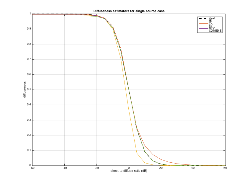
---Sigle source case
In the basic mixture of a single point/plane wave source, and an isotropic diffuse field, all estimators perform well. More specifically the IE, DPV, and COMEDIE estimators give perfect results, if enough observations are taken so that the statistics are captured properly. The SV and TV estimators have a small bias, the SV underestimates diffuseness and TV overestimates slightly. The example below demonstrates this case.
aziElev2aziPolar = @(dirs) [dirs(:,1) pi/2-dirs(:,2)]; % function to convert from azimuth-inclination to azimuth-elevation
% direct-to-reverberant ratio for test cases
ddr_db = (-60:5:60)';
ddr = 10.^(ddr_db/10);
% ideal diffuseness
diff_ideal = 1./(1+ddr);

% source signal modeling
lSig = 10000; % observations
src_dirs = [0 0];
nSrc = size(src_dirs,1);
Ps = 1; % unit power source
srcsig = sqrt(Ps)*exp(1i*pi*(2*rand(nSrc, lSig)-1)); % model direct sound as complex exponentials with uniformly distributed random phase
order = 2;
nSH = (order+1)^2;
Y_src = getSH(order, aziElev2aziPolar(src_dirs), 'real'); % direct sound incident from front
A_dir = Y_src';
sh_dirsig = A_dir*srcsig; % SH signals for direct sound
% diffuse signal modeling
[~, diff_dirs] = getTdesign(21); % get dense uniform distribution of directions
nDiff = size(diff_dirs,1);
diffsig = sqrt(1/nDiff)*exp(1i*pi*(2*rand(nDiff, lSig)-1)); % model diffuse sound as complex exponentials with uniformly distributed random phase
Y_diff = getSH(order, aziElev2aziPolar(diff_dirs), 'real');
A_diff = Y_diff';
sh_diffsig_ref = A_diff*diffsig; % SH signals for unit power diffuse sound
% transformation matrix from SH signals to pressure velocity signals
M_sh2pv = beamWeightsPressureVelocity('real');

% compute diffuseness for varying DDR
diff_ie = zeros(length(ddr),1);
diff_tv = zeros(length(ddr),1);
diff_sv = zeros(length(ddr),1);
diff_dpv = zeros(length(ddr),1);
diff_comedie = zeros(length(ddr),1);
for nd=1:length(ddr)

    % adjust power of diffuse sound
    Pdiff = Ps/ddr(nd); % power of diffuse sound
    sh_diffsig = sqrt(Pdiff)*sh_diffsig_ref;
    % SH signals
    shsig = sh_dirsig+sh_diffsig;
    % Pressure-velocity signals
    pvsig = M_sh2pv*shsig(1:4,:);
    % Intensity vector signals (actually they point to DoA instead of propagation as in the usual acoustic intensity convention)
    isig = real( (ones(3,1)*pvsig(1,:)) .* conj(pvsig(2:4,:)) )';
    % correlations of SH signals
    sphCOV = (1/lSig) * (shsig*shsig');
    % correlations of PV signals
    pvCOV = (1/lSig) * (pvsig*pvsig');

    % Intensity-energy density ratio
    diff_ie(nd) = getDiffuseness_IE(pvCOV); % compute diffuseness

    % Temporal variation of intensity vectors
    diff_tv(nd) = getDiffuseness_TV(isig);

    % Spherical variance of intensity DoAs
    diff_sv(nd) = getDiffuseness_SV(isig);

    % Directional power variance SHD diffuseness estimator
    diff_dpv(nd) = getDiffuseness_DPV(sphCOV);

    % COMEDIE SHD diffuseness estimator
    diff_comedie(nd) = getDiffuseness_CMD(sphCOV);

end
figure
plot(ddr_db, diff_ideal, '--k','linewidth',2)
hold on, plot(ddr_db, [diff_ie diff_tv diff_sv diff_dpv diff_comedie]), grid, legend('ideal','IE','TV','SV', 'DPV', 'COMEDIE')
title('Diffuseness estimators for single source case'), xlabel('direct-to-diffuse ratio (dB)'), ylabel('diffuseness')
h = gcf; h.Position(3) = 1.5*h.Position(3); h.Position(4) = 1.5*h.Position(4);
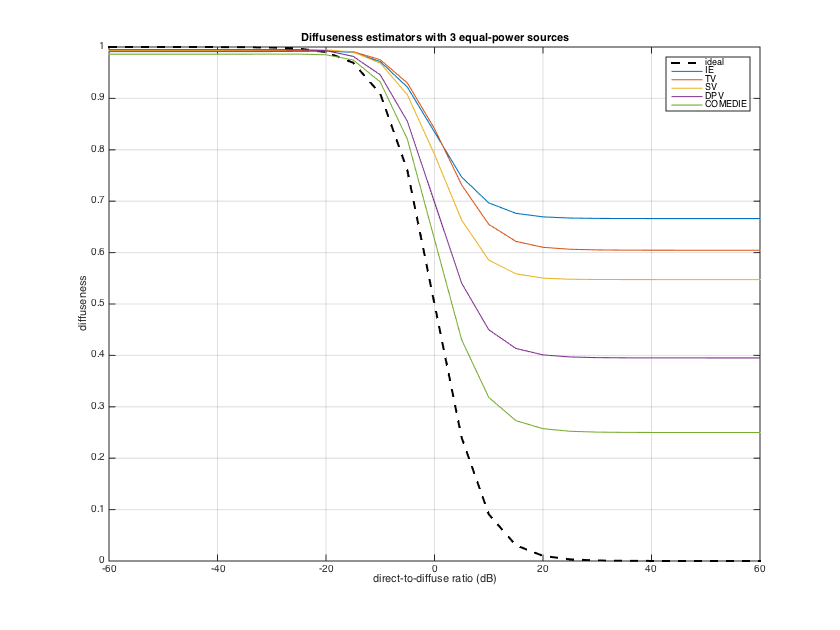
---Multiple sources case
The simplest of the above estimators, the IE, SV and TV, that use only the first-order signals, are limited in their ability to assess diffuseness in the presence of more than one source, overestimating diffuseness. To get a better estimate in this case, the higher-order signals can be used if available. The more advanced estimators such as the DPV and COMEDIE exploit the higher spatial resolution of the higher-order signals and give a closer estimate to the true diffuseness/DDR for multiple sources, when the sources are less than the number of SH signals. Note that the DPV, however, similar to the first-order estimators, overestimates diffuseness in the presence of correlated sources, something that the COMEIDE estimator is robust against.
% source signal modeling
lSig = 10000; % samples
src_dirs = [0 0; pi 0; -pi/2 pi/4];
nSrc = size(src_dirs,1);
Ps = [1 1 1]; % unit power sources
srcsig = diag(sqrt(Ps))*exp(1i*pi*(2*rand(nSrc, lSig)-1)); % model direct sound as complex exponentials with uniformly distributed random phase
order = 2;
nSH = (order+1)^2;
Y_src = getSH(order, aziElev2aziPolar(src_dirs), 'real');
A_dir = Y_src';
sh_dirsig = A_dir*srcsig; % SH signals for direct sound
% diffuse signal modeling
[~, diff_dirs] = getTdesign(21); % get dense uniform distribution of directions
nDiff = size(diff_dirs,1);
diffsig = sqrt(1/nDiff)*exp(1i*pi*(2*rand(nDiff, lSig)-1)); % model diffuse sound as complex exponentials with uniformly distributed random phase
Y_diff = getSH(order, aziElev2aziPolar(diff_dirs), 'real');
A_diff = Y_diff';
sh_diffsig_ref = A_diff*diffsig; % SH signals for unit power diffuse sound
% transformation matrix from SH signals to pressure velocity signals
M_sh2pv = beamWeightsPressureVelocity('real');

% compute diffuseness for varying DDR
diff_ie = zeros(length(ddr),1);
diff_tv = zeros(length(ddr),1);
diff_sv = zeros(length(ddr),1);
diff_dpv = zeros(length(ddr),1);
diff_comedie = zeros(length(ddr),1);
for nd=1:length(ddr)

    % adjust power of diffuse sound
    Pdiff = sum(Ps)/ddr(nd); % power of diffuse sound
    sh_diffsig = sqrt(Pdiff)*sh_diffsig_ref;
    % SH signals
    shsig = sh_dirsig+sh_diffsig;
    % Pressure-velocity signals
    pvsig = M_sh2pv*shsig(1:4,:);
    % Intensity vector signals (actually they point to DoA instead of propagation as in the usual acoustic intensity convention)
    isig = real( (ones(3,1)*pvsig(1,:)) .* conj(pvsig(2:4,:)) )';
    % correlations of SH signals
    sphCOV = (1/lSig) * (shsig*shsig');
    % correlations of PV signals
    pvCOV = (1/lSig) * (pvsig*pvsig');

    % Intensity-energy density ratio
    diff_ie(nd) = getDiffuseness_IE(pvCOV); % compute diffuseness

    % Temporal variation of intensity vectors
    diff_tv(nd) = getDiffuseness_TV(isig);

    % Spherical variance of intensity DoAs
    diff_sv(nd) = getDiffuseness_SV(isig);

    % Directional power variance SHD diffuseness estimator
    diff_dpv(nd) = getDiffuseness_DPV(sphCOV);

    % COMEDIE SHD diffuseness estimator
    diff_comedie(nd) = getDiffuseness_CMD(sphCOV);

end
figure
plot(ddr_db, diff_ideal, '--k','linewidth',2)
hold on, plot(ddr_db, [diff_ie diff_tv diff_sv diff_dpv diff_comedie]), grid, legend('ideal','IE','TV','SV', 'DPV', 'COMEDIE')
title('Diffuseness estimators with 3 equal-power sources'), xlabel('direct-to-diffuse ratio (dB)'), ylabel('diffuseness')
h = gcf; h.Position(3) = 1.5*h.Position(3); h.Position(4) = 1.5*h.Position(4);
DIFFUSE-FIELD COHERENCE OF DIRECTIONAL SENSORS/BEAMFORMERS [ref.8]
The diffuse-field coherence (DFC) matrix, under isotropic diffuse conditions, is a fundamental quantity in acoustical array processing, since it models approximately the second-order statistics of late reverberant sound, and is useful in a wide variety of beamforming and dereverberation tasks. The DFC matrix expresses the PSD matrix between the array sensors, or beamformers, for a diffuse-sound field, normalized with the diffuse sound power, and it depends only on the properties of the microphones, directionality, orientation and position in space.
Analytic expressions for the DFC exist only for omnidirectional sensors at arbitrary positions, the well-known sinc function of the wavenumber-distance product, and for first-order directional microphones with arbitrary orientations, see e.g. [ref18]. For more general directivities, [ref.8] shows that the DCM can be pre-computed through the expansion of the microphone/beamformer patterns into SHD coefficients.
The example code below demonstrates this method for a number of cases:
clear all; close all;
% inline function to convert from azimuth-inclination to azimuth-elevation
aziElev2aziPolar = @(dirs) [dirs(:,1) pi/2-dirs(:,2)];
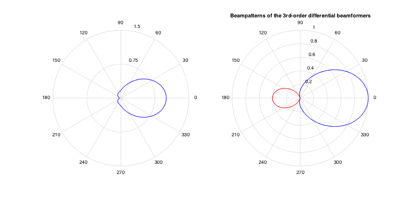
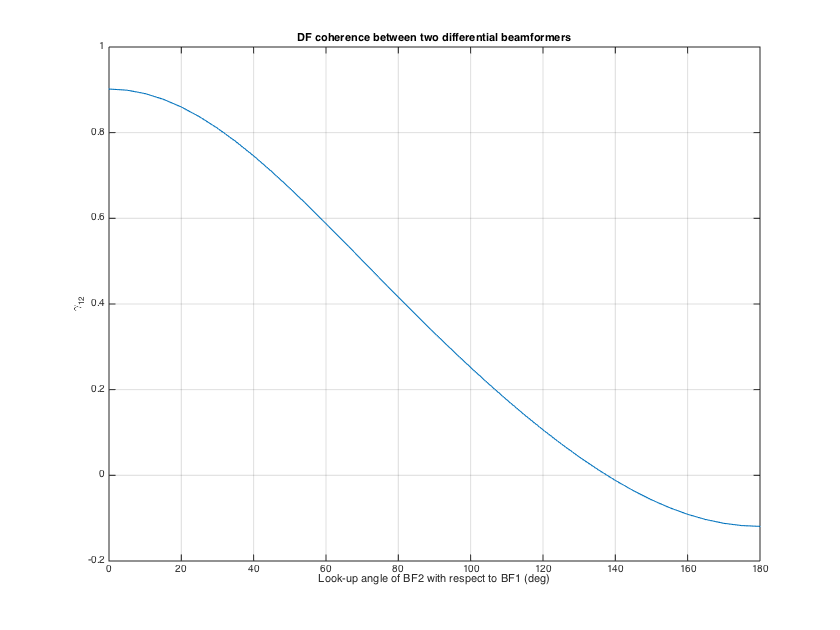
---DFC between two coincident beamformers/sensors
In this case two beamformers are described by beamforming weights in the SHD. The DFC is directly given by the dot-product of the beamforming weights.
% inline function for coincident DFC from SHD coefficients
dfc_coinc = @(coeff_set1, coeff_set2, minOrder) (coeff_set1(1:(minOrder+1)^2)'*coeff_set2(1:(minOrder+1)^2))/sqrt( sum(abs(coeff_set1).^2) * sum(abs(coeff_set2).^2) );

% define two third-order beamformers of the differential form
order = 3;
w_df1 = [0.174, 0.207, 0.343, 0.277]'; w_df1 = w_df1/sum(w_df1);
w_df2 = [0.112, 0.357, 0.184, 0.347]'; w_df2 = w_df2/sum(w_df2);
% convert to SHD weights
w_shd1 = beamWeightsDifferential2Spherical(w_df1);
w_shd2 = beamWeightsDifferential2Spherical(w_df2);
% plot beampatterns
figure, h_ax = subplot(121); plotAxisymPatternFromCoeffs(w_shd1, h_ax);
h_ax = subplot(122); plotAxisymPatternFromCoeffs(w_shd2, h_ax);
title('Beampatterns of the 3rd-order differential beamformers')
h = gcf; h.Position(3) = 1.5*h.Position(3);
% rotate the second pattern from 0 to 180deg, and compute the DFC
% between the two patterns for each angle
theta = (0:5:180)'*pi/180;
dfc_12 = zeros(size(theta));
w_shd1_0 = rotateAxisCoeffs(w_shd1,0,0,'real'); % go from (N+1) to (N+1)^2 coeffs without rotation, fill with zeros
for nt=1:length(theta)
    w_shd2_rot = rotateAxisCoeffs(w_shd2,theta(nt),0,'real'); % rotate second axisymmetric pattern

    dfc_12(nt) = dfc_coinc(w_shd1_0, w_shd2_rot, order);
end
figure, plot(theta*180/pi, dfc_12), grid
title('DF coherence between two differential beamformers')
xlabel('Look-up angle of BF2 with respect to BF1 (deg)'), ylabel('\gamma_{12}')
h = gcf; h.Position(3) = 1.5*h.Position(3); h.Position(4) = 1.5*h.Position(4);
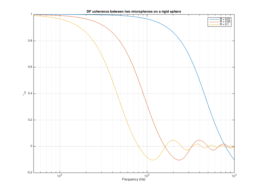
---DFC matrix of microphones on sphere
In the case that the array response is known analytically as an expansion in the SHD, e.g. for microphones on a rigid sphere, the DFC matrix can be computed directly following a similar approach as above. This case is suitable when the expansion consider the overall response of each sensor in the global array coordinates, including their phase response with respect to the phase center of the array. This case is also suitable when an array response has been measured in multiple directions around a measurement center, and then is subsequently expanded into SH coefficients, see [ref8] for details. An example of such a case are HRTF measurements.
% simulate array response of a tetrahedral array on a rigid sphere for 3
% different radius
[~, mic_dirs_rad] = getTdesign(2);
nMics = 4;
c = 343;
f = (0:10:10000);
R = [0.01 0.05 0.1];
for nr=1:length(R)
    kR = 2*pi*f*R(nr)/c;
    kR_max = kR(end);
    order_array = ceil(kR_max);
    Y_array = sqrt(4*pi)*getSH(order_array, aziElev2aziPolar(mic_dirs_rad), 'real');
    % modal responses
    bN = sphModalCoeffs(order_array, kR, 'rigid')/(4*pi);
    % array response in the SHD and DFC matrix
    H_array = zeros(nMics, (order_array+1)^2, length(f));
    DFCmtx = zeros(nMics,nMics, length(f));
    for kk=1:length(f)
        temp_b = bN(kk,:).';
        B = diag(replicatePerOrder(temp_b));
        H_array(:,:,kk) = Y_array*B;

        DFCmtx(:,:,kk) = H_array(:,:,kk)*H_array(:,:,kk)';
    end
    % coherence betwen sensor 1 and 4 (should be real)
    dfc_14(:,nr) = squeeze( DFCmtx(1,4,:)./sqrt( DFCmtx(1,1,:) .* DFCmtx(4,4,:) ) );
end
figure, semilogx(f, real(dfc_14)), set(gca, 'xlim',[50 10000]), grid
legend(['R = ' num2str(R(1))],['R = ' num2str(R(2))],['R = ' num2str(R(3))])
title('DF coherence between two microphones on a rigid sphere')
xlabel('Frequency (Hz)'), ylabel('\gamma_{14}')
h = gcf; h.Position(3) = 1.5*h.Position(3); h.Position(4) = 1.5*h.Position(4);
clear H_array B bN% clear some large space
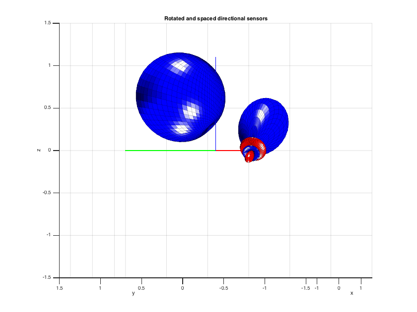
---DFC between spaced directional sensors with arbitrary directivity
When the directional response of two individual microphones is known, their DFC may be needed for some arbitrary spacing and orientation of the sensors. This case is more complex than the previous one, and it involves a plane-wave expansion and the product of the two patterns in the SHD, as shown in [ref8].
% assume two sensors, one with a 2nd-order cardioid response, and another
% with 3rd-order supercardioid
w1 = beamWeightsCardioid2Spherical(2);
w2 = beamWeightsHypercardioid2Spherical(3);
% orient the two microphones at (azi,elev) [pi/2 pi/4] and [0 pi/6] respectively.
azi1 = pi/2; incl1 = pi/2-pi/4; % go from elev to inclination
azi2 = 0; incl2 = pi/2-pi/6;
w1_rot = rotateAxisCoeffs(w1, incl1, azi1, 'real');
w2_rot = rotateAxisCoeffs(w2, incl2, azi2, 'real');
% define position of sensors in meters
r1 = [0 0.1 0.3];
r2 = [-0.2 -0.5 -0];
% plot patterns
figure, h_ax = gca;
plotSphFunctionCoeffs(w1_rot, 'real', 5, 5, 'real', h_ax)
plotSphFunctionCoeffs(w2_rot, 'real', 5, 5, 'real', h_ax), grid
% translate pattern to its location by getting pattern handles
h_surf = findobj(gca,'Type','Surface');
h_surf(1).XData = h_surf(1).XData + r2(1); h_surf(1).YData = h_surf(1).YData + r2(2); h_surf(1).ZData = h_surf(1).ZData + r2(3);
h_surf(2).XData = h_surf(2).XData + r2(1); h_surf(2).YData = h_surf(2).YData + r2(2); h_surf(2).ZData = h_surf(2).ZData + r2(3);
h_surf(3).XData = h_surf(3).XData + r1(1); h_surf(3).YData = h_surf(3).YData + r1(2); h_surf(3).ZData = h_surf(3).ZData + r1(3);
h_surf(4).XData = h_surf(4).XData + r1(1); h_surf(4).YData = h_surf(4).YData + r1(2); h_surf(4).ZData = h_surf(4).ZData + r1(3);
axis([-1.5 1.5 -1.5 1.5 -1.5 1.5]), view(-75,0); title('Rotated and spaced directional sensors')
h = gcf; h.Position(3) = 1.5*h.Position(3); h.Position(4) = 1.5*h.Position(4);
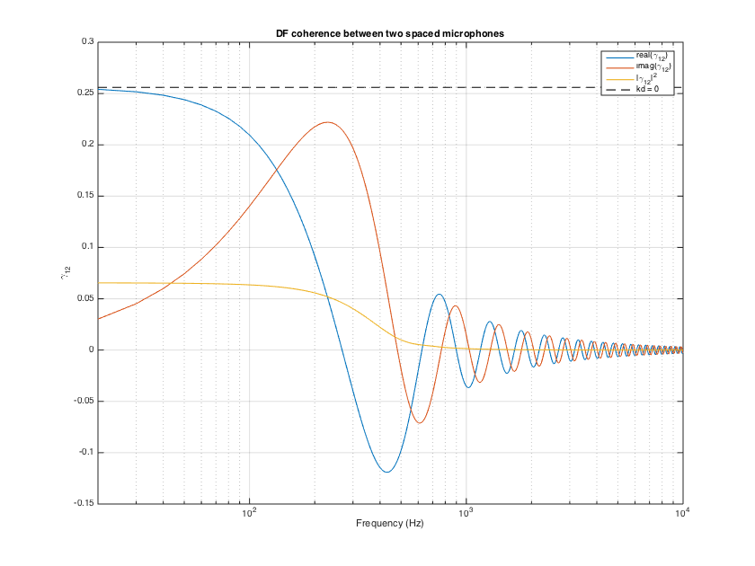
% frequency vector to compute DFC
f = (0:10:10000)';
c = 343;
k = 2*pi*f/c;
% compute DFC (SLOW FOR HIGH ORDERS!!! TODO: use pre-computed Gaunt coefficients)
dfc_12 = diffCoherence(k, r1, r2, real2complexCoeffs(w1_rot), real2complexCoeffs(w2_rot)); % multiplication defined for complex SH coeffs (TODO: real SH multiplication)
% compute DFC for zero distance between sensors for comparison
minOrder = 2;
dfc_12_r0 = dfc_coinc(w1_rot, w2_rot, minOrder);
% plot results
figure, semilogx(f, [real(dfc_12) imag(dfc_12) abs(dfc_12).^2])
line(f,ones(size(f))*dfc_12_r0,'linestyle','--','color','k')
set(gca, 'xlim',[20 10000]), grid, legend('real(\gamma_{12})','imag(\gamma_{12})','|\gamma_{12}|^2','kd = 0')
title('DF coherence between two spaced microphones')
xlabel('Frequency (Hz)'), ylabel('\gamma_{12}')
h = gcf; h.Position(3) = 1.5*h.Position(3); h.Position(4) = 1.5*h.Position(4);
REFERENCES
1.  Moreau, S., Daniel, J., Bertet, S., 2006,
    3D sound field recording with higher order ambisonics-objective measurements and validation of spherical microphone.
    In Audio Engineering Society Convention 120.
2. Mh Acoustics Eigenmike, https://mhacoustics.com/products#eigenmike1
3.  Bernsch?tz, B., P?rschmann, C., Spors, S., Weinzierl, S., Verst?rkung, B., 2011.
    Soft-limiting der modalen amplitudenverst?rkung bei sph?rischen mikrofonarrays im plane wave decomposition verfahren.
    Proceedings of the 37. Deutsche Jahrestagung f?r Akustik (DAGA 2011)
4.  Jin, C.T., Epain, N. and Parthy, A., 2014.
    Design, optimization and evaluation of a dual-radius spherical microphone array.
    IEEE/ACM Transactions on Audio, Speech, and Language Processing, 22(1), pp.193-204.
5.  Elko, G.W., 2004. Differential microphone arrays.
    In Audio signal processing for next-generation multimedia communication systems (pp. 11-65). Springer.
6.  Zotter, F., Pomberger, H. and Noisternig, M., 2012.
    Energy-preserving ambisonic decoding. Acta Acustica united with Acustica, 98(1), pp.37-47.
7.  Koretz, A. and Rafaely, B., 2009.
    Dolph?Chebyshev beampattern design for spherical arrays.
    IEEE Transactions on Signal Processing, 57(6), pp.2417-2420.
8.  Politis, A., 2016.
    Diffuse-field coherence of sensors with arbitrary directional responses. arXiv preprint arXiv:1608.07713.
9.  Hafizovic, I., Nilsen, C.I.C. and Holm, S., 2012.
    Transformation between uniform linear and spherical microphone arrays with symmetric responses.
    IEEE Transactions on Audio, Speech, and Language Processing, 20(4), pp.1189-1195.
10. Politis, A. and Pulkki, V., 2016.
    Acoustic intensity, energy-density and diffuseness estimation in a directionally-constrained region.
    arXiv preprint arXiv:1609.03409.
11. Thiergart, O. and Habets, E.A., 2014.
    Extracting reverberant sound using a linearly constrained minimum variance spatial filter.
    IEEE Signal Processing Letters, 21(5), pp.630-634.
12. Thiergart, O., Taseska, M. and Habets, E.A., 2014.
    An informed parametric spatial filter based on instantaneous direction-of-arrival estimates.
    IEEE/ACM Transactions on Audio, Speech, and Language Processing, 22(12), pp.2182-2196.
13. Merimaa, J. and Pulkki, V., 2005.
    Spatial impulse response rendering I: Analysis and synthesis.
    Journal of the Audio Engineering Society, 53(12), pp.1115-1127.
14. Ahonen, J. and Pulkki, V., 2009.
    Diffuseness estimation using temporal variation of intensity vectors.
    In 2009 IEEE Workshop on Applications of Signal Processing to Audio and Acoustics (WASPAA).
15. Politis, A., Delikaris-Manias, S. and Pulkki, V., 2015.
    Direction-of-arrival and diffuseness estimation above spatial aliasing for symmetrical directional microphone arrays.
    In 2015 IEEE International Conference on Acoustics, Speech and Signal Processing (ICASSP).
16. Gover, B.N., Ryan, J.G. and Stinson, M.R., 2002.
    Microphone array measurement system for analysis of directional and spatial variations of sound fields.
    The Journal of the Acoustical Society of America, 112(5), pp.1980-1991.
17. Epain, N. and Jin, C.T., 2016.
    Spherical Harmonic Signal Covariance and Sound Field Diffuseness.
    IEEE/ACM Transactions on Audio, Speech, and Language Processing, 24(10), pp.1796-1807.
18. Elko, G.W., 2001.
    Spatial coherence functions for differential microphones in isotropic noise fields.
    In Microphone Arrays (pp. 61-85). Springer Berlin Heidelberg.