Otto Mikkonen, Alec Wright, Eloi Moliner and Vesa Välimäki
Companion page for a paper in the the 26th International Conference on Digital Audio Effects (DAFx23) Copenhagen, Denmark, September, 2023
A pre-print of the article is available in arXiv.
The datasets can be downloaded from Zenodo.
The code is open-source and published in Github.
Abstract
The sound of magnetic recording media, such as open reel and cassette tape recorders, is still sought after by today's sound practitioners due to the imperfections embedded in the physics of
the magnetic recording process.
This paper proposes a method for digitally emulating this character using neural networks.
The signal chain of the proposed system consists of three main components: the hysteretic nonlinearity and filtering jointly produced by the magnetic recording process as well as the record
and playback amplifiers, the fluctuating delay originating from the tape transport, and the combined additive noise component from various electromagnetic origins.
In our approach, the hysteretic nonlinear block is modeled using a recurrent neural network, while the delay trajectories and the noise component are generated using separate diffusion models,
which employ U-net deep convolutional neural networks.
According to the conducted objective evaluation, the proposed architecture faithfully captures the character of the magnetic tape recorder.
The results of this study can be used to construct virtual replicas of vintage sound recording devices.
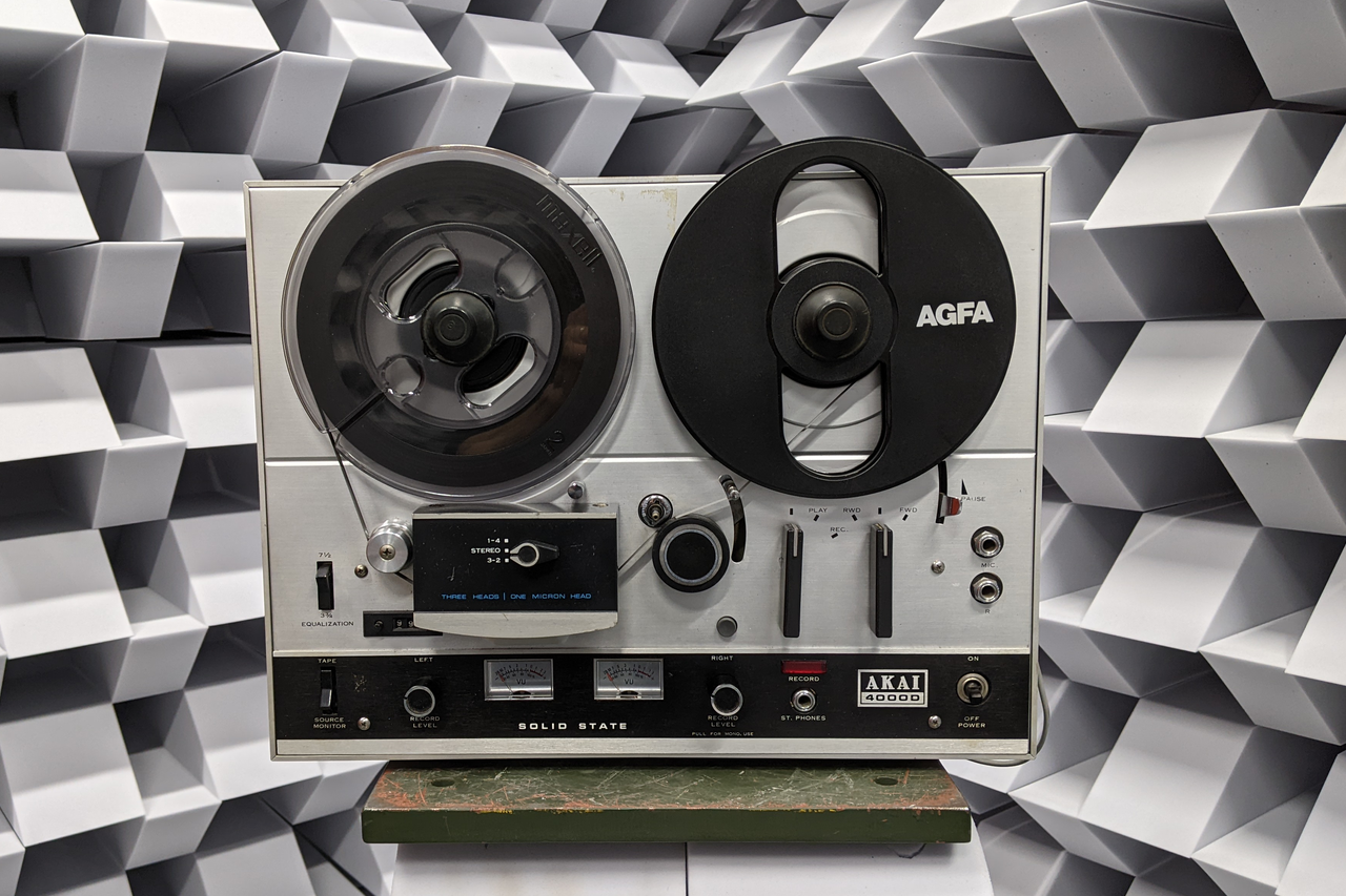
Figure 1: AKAI 4000D open reel tape recorder.
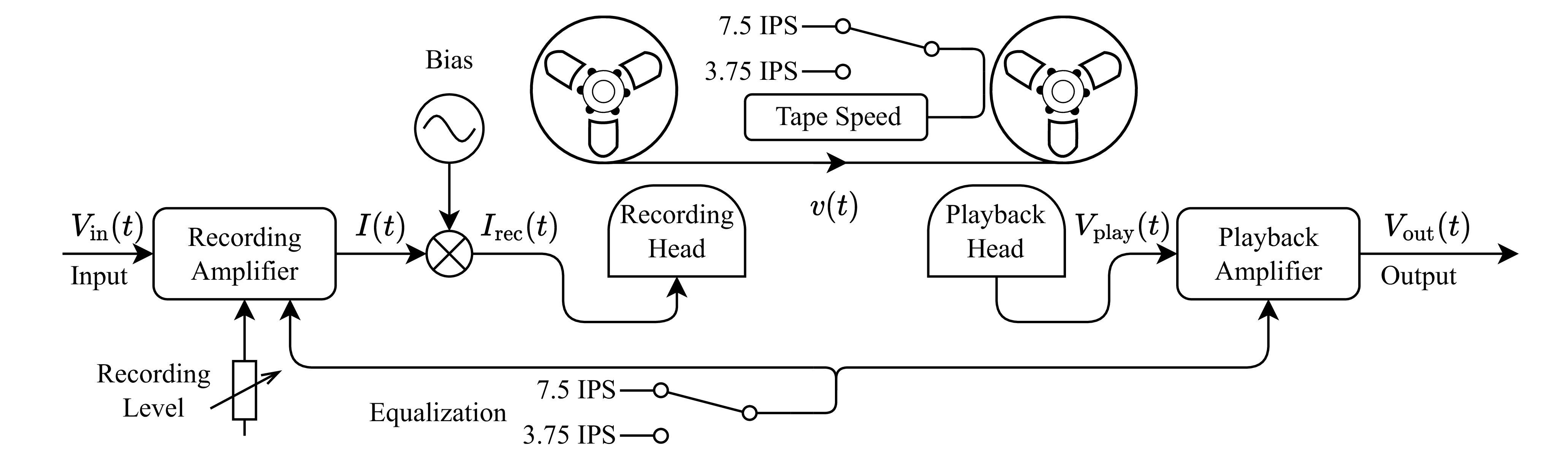
Target System Block Diagram
The block diagram of a typical magnetic recorder is shown in Fig. 2.
Figure 2: Target system block diagram.
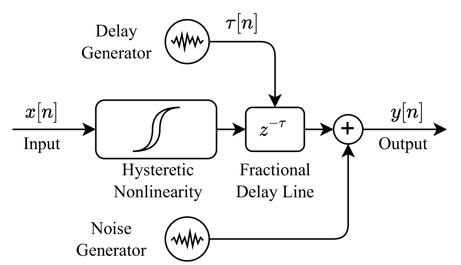
Modeling Architecture
The grey-box architecture used for the modeling is shown in Fig. 3.
Figure 3: Modeling architecture.
Experiment 1 - Toy Data
In this section, the proposed system is evaluated using synthetic data.
The data is generated by processing a fraction of the inputs from the SignalTrain dataset using a VST instance of CHOWTape, a white-box tape machine model.
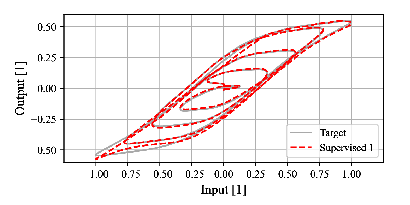
Lumped nonlinearities only
The model hysteresis curve versus the target is shown in Fig. 4.
Audio examples from the experiment are provided in the table underneath.
Figure 4: Model hysteresis using toy data - Lumped nonlinearities only.
Input
Target
Supervised I
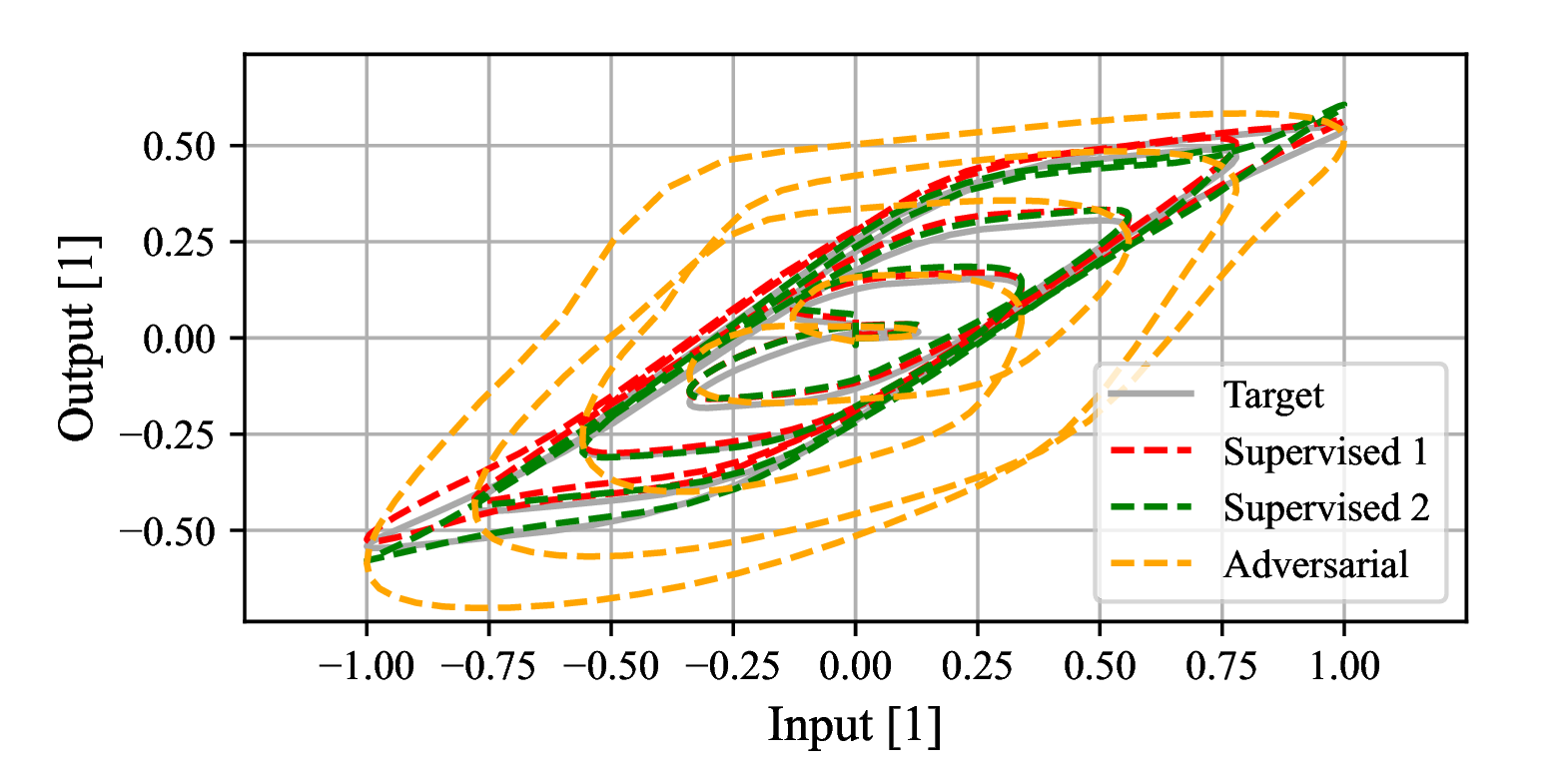
Lumped nonlinearities and timing effects
The hysteresis curves of the models trained using the three approaches versus the target is shown in Fig. 5.
Audio examples from the experiment are provided in the table underneath.
Figure 5: Model hysteresis using toy data - Nonlinearities and timing effects.
Input
Target
Supervised I
Supervised II
Adversarial
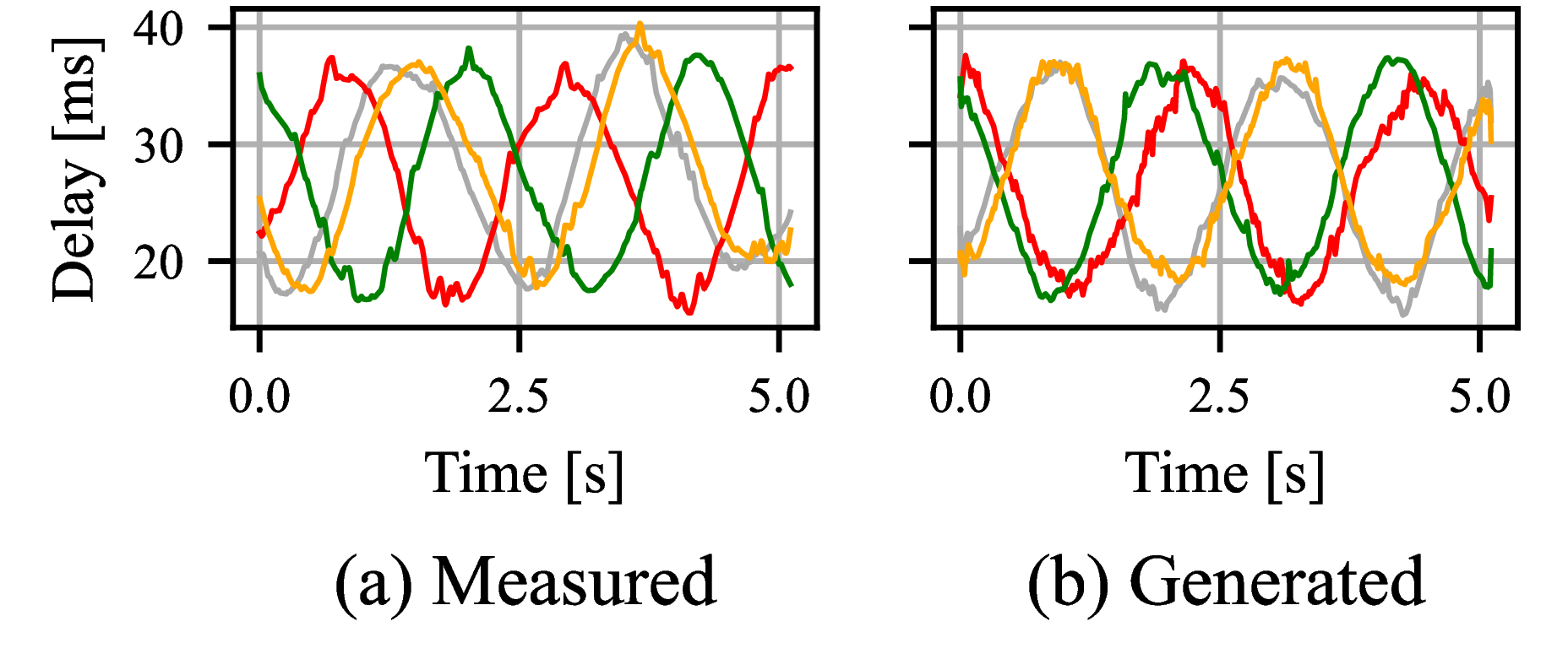
Trajectory generator
Fig. 6 shows a qualitative comparison between measured and generated delay trajectories.
Figure 6: Plots of measured and generated delay trajectories in (left) time and (right) frequency domains using toy data.
Full model
This section demonstrates the performance of the modeling architecture without the noise component,
consisting of the trained nonlinear block and the trajectory generator.
As a demonstration, we compare the model prediction to ground truth by applying as a delay trajectory either
the true trajectory (Pred. + True traj.)
a trajectory from the generative model (Pred. + Gen. traj.).
We use the best model from Sec. 'Lumped nonlinearities and timing effects' for the nonlinearities.
Input
Target
Pred. + True traj.
Pred. + Gen. traj. 1
Pred. + Gen. traj. 2
Experiment 2 - Real Data
In this section, the proposed system is evaluated using real data collected from the Akai 4000D open-reel tape recorder (Fig. 1).
We use the same input audio as in previous section.
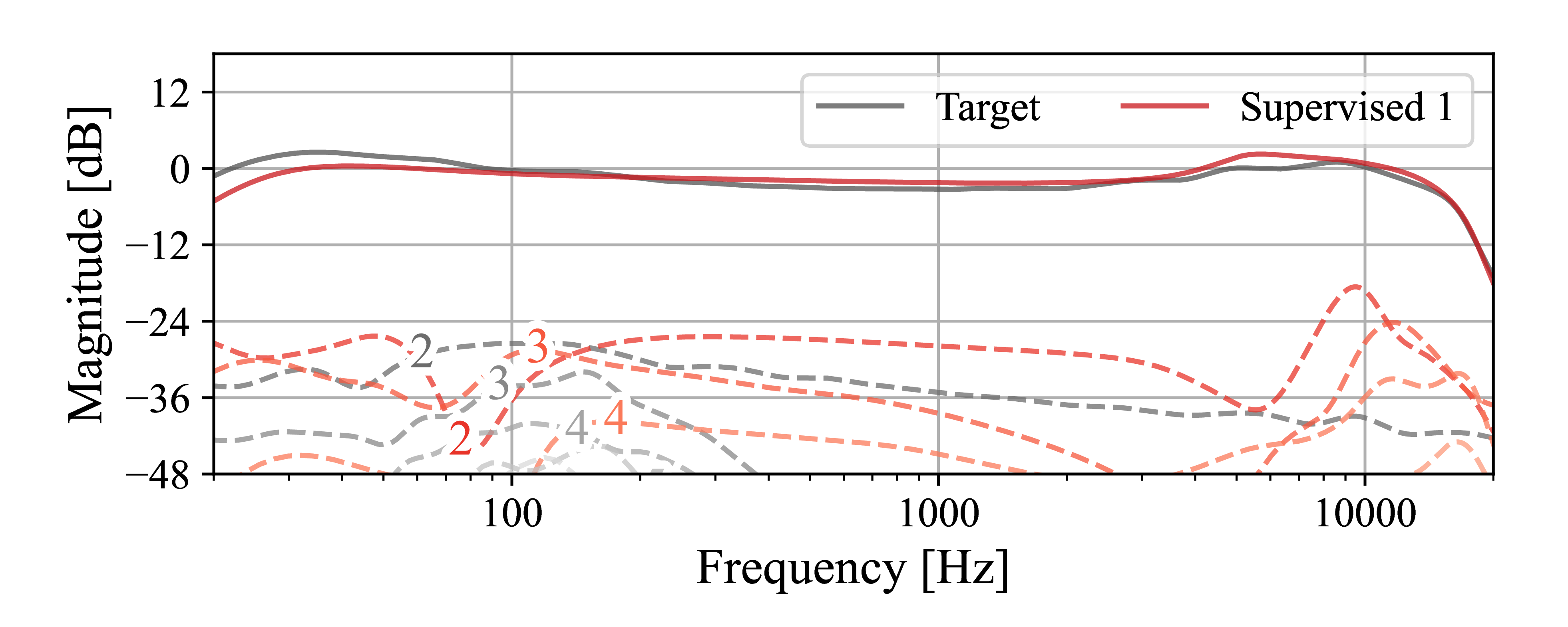
Lumped nonlinearities and timing effects
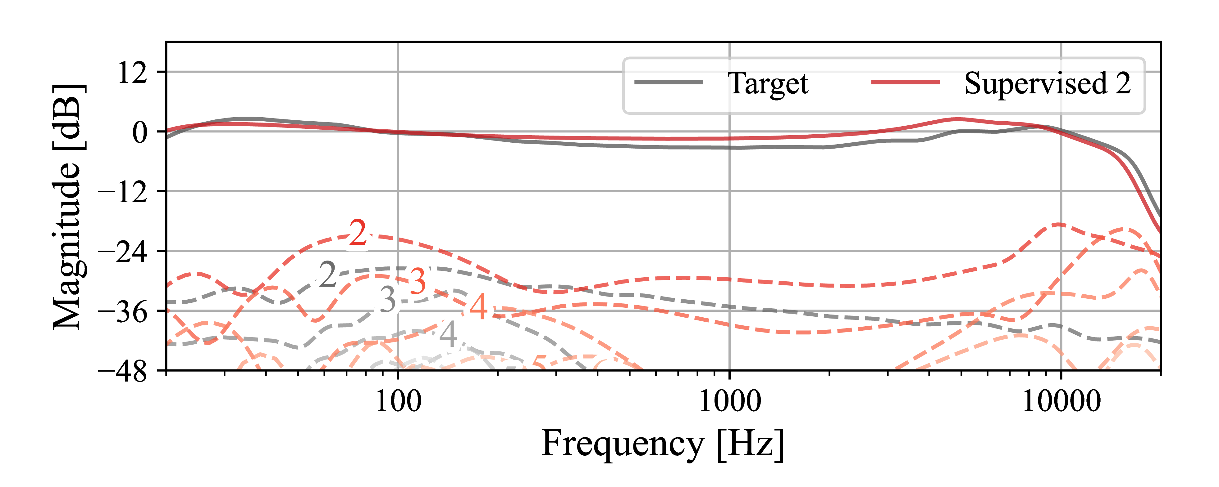
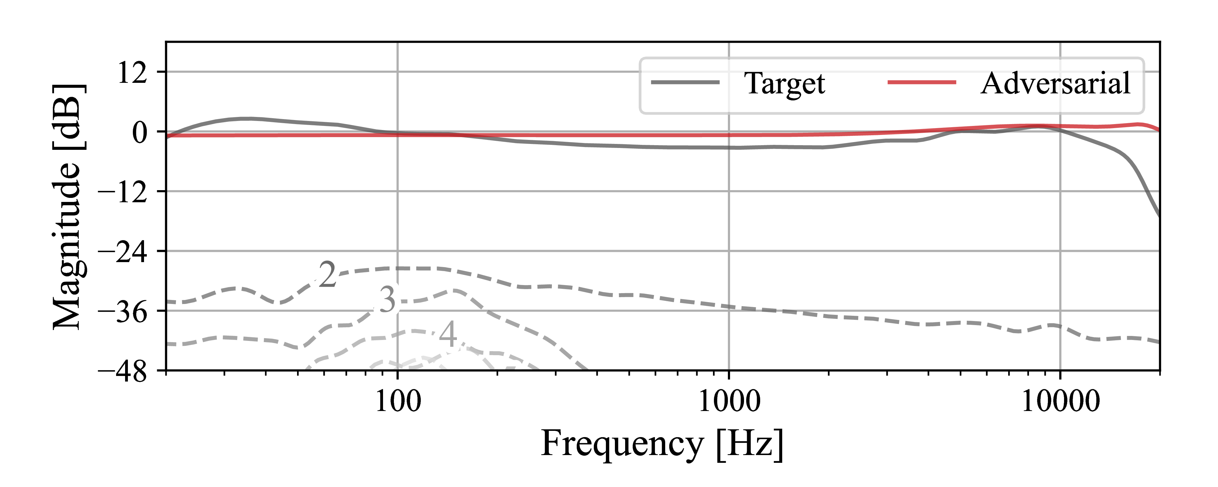
The learned magnitude responses and nonlinear distortion components produced by the models versus the target is shown in Fig. 7.
Audio examples from the experiment are provided in the table underneath. The model predictions are summed together with a noise component from the real distribution.
Supervised I.
Supervised II.
Adversarial.
Figure 7: Model magnitude responses (solid) and distortion components (dashed), MAXELL 7.5IPS.
Input
Target
Supervised I
Supervised II
Adversarial
Trajectory generator
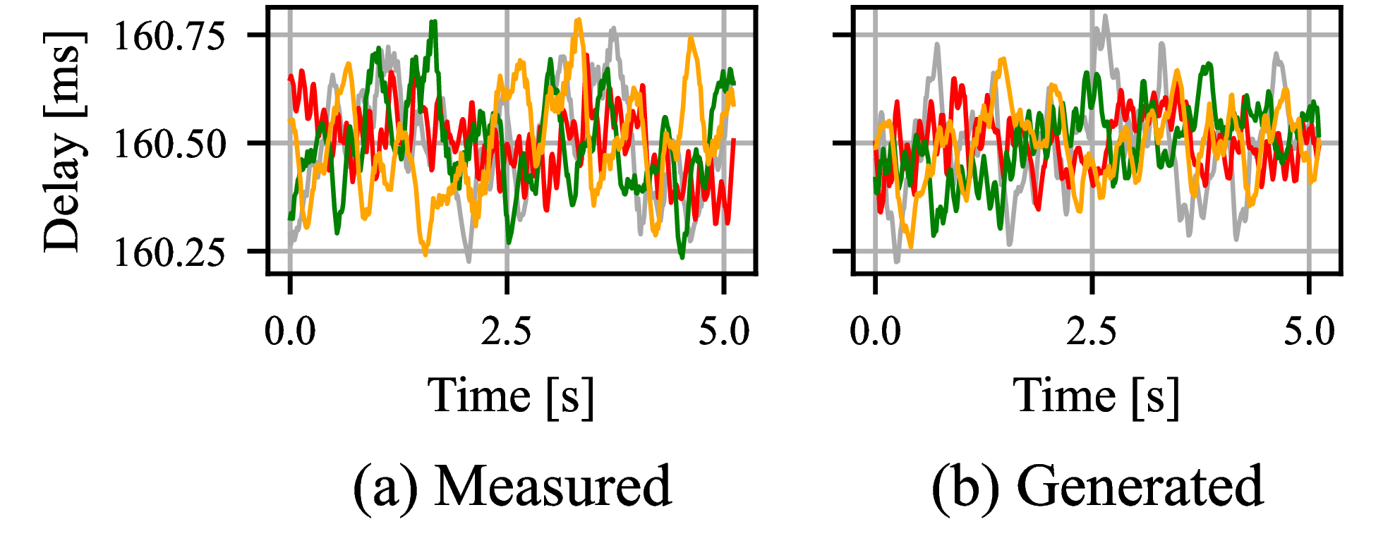
Fig. 8 shows a qualitative comparison between measured and generated delay trajectories.
Figure 8: Plots of measured and generated delay trajectories in (left) time and (right) frequency domains using real data.
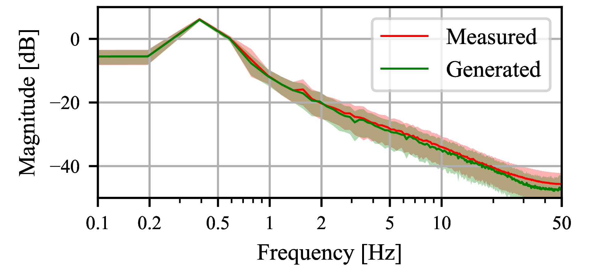
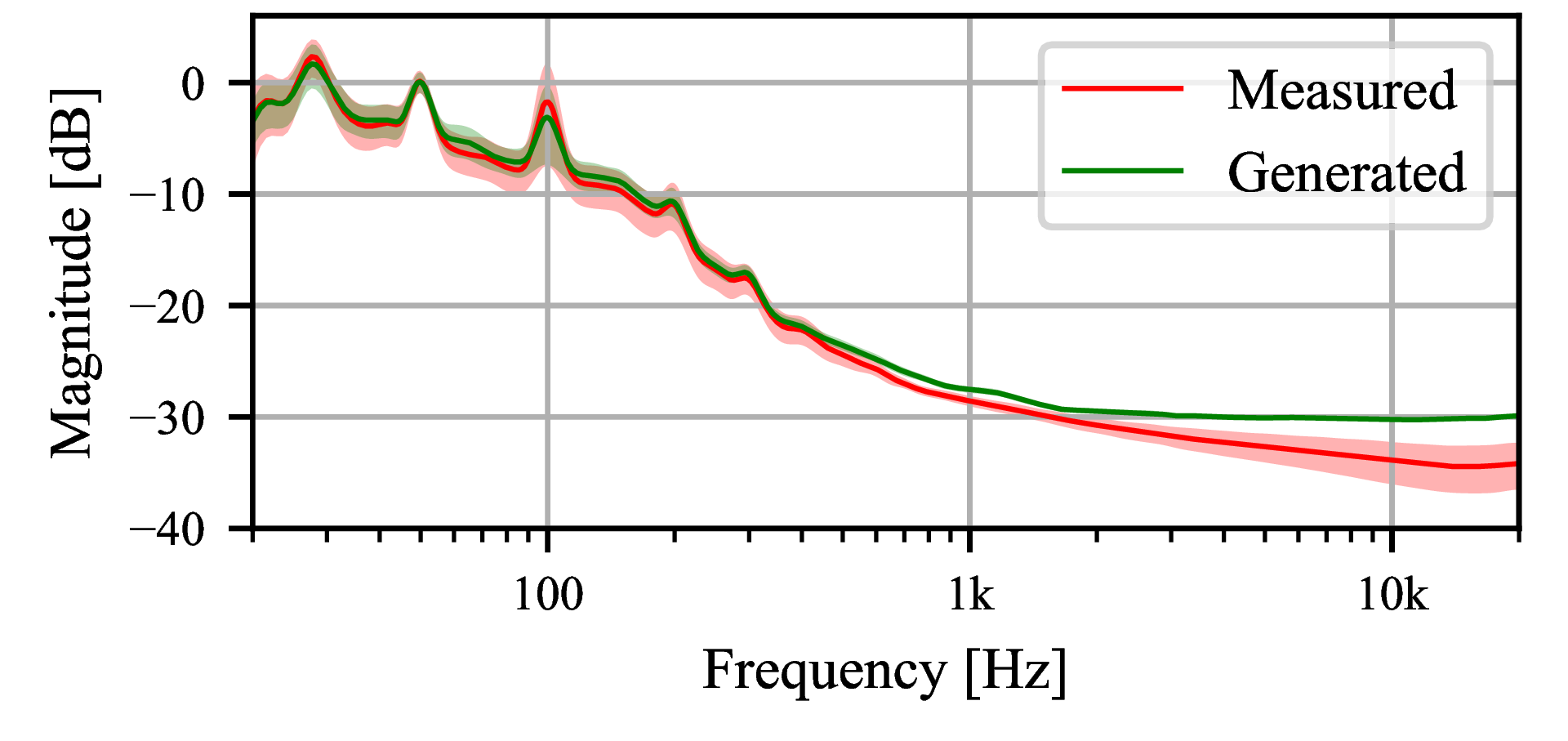
Noise generator
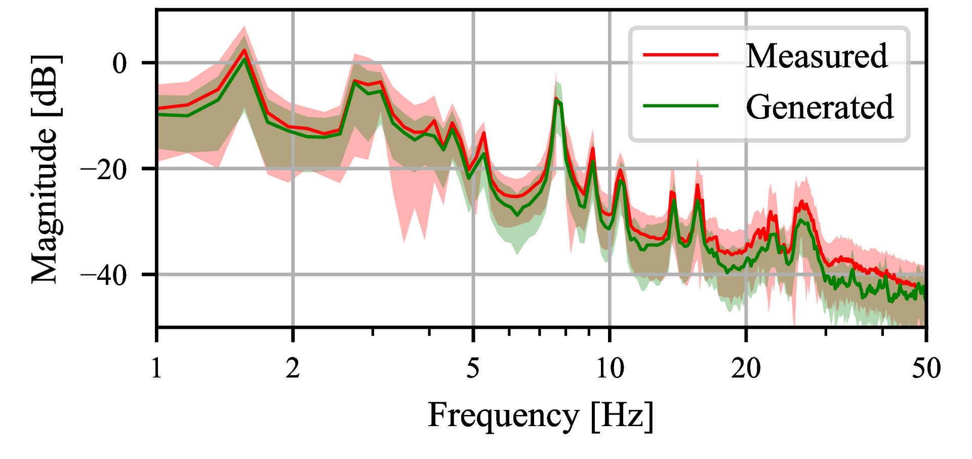
The statistics of the generated noise component versus the ground truth is shown in Fig. 9.
Audio examples from the experiment are provided in the table underneath.
Figure 9: Statistics of measured and synthetic tape hiss generated by a diffusion model.
Real
Generated
Full model
This section demonstrates the performance of the modeling architecture using real data.
As a demonstration, we compare the model prediction to ground truth by applying a noise component from either
the real distribution (Pred. + Real Noise.)
the generative model (Pred. + Gen. Noise.).
We use the best model from Sec. 'Lumped nonlinearities and timing effects' for the nonlinearities.