Archontis Politis and Juha Vilkamo and Ville Pulkki

Sector-Based Parametric Sound Field Reproduction in the Spherical Harmonic Domain

Acoustic velocity beamforming in a spatially-filtered sound field

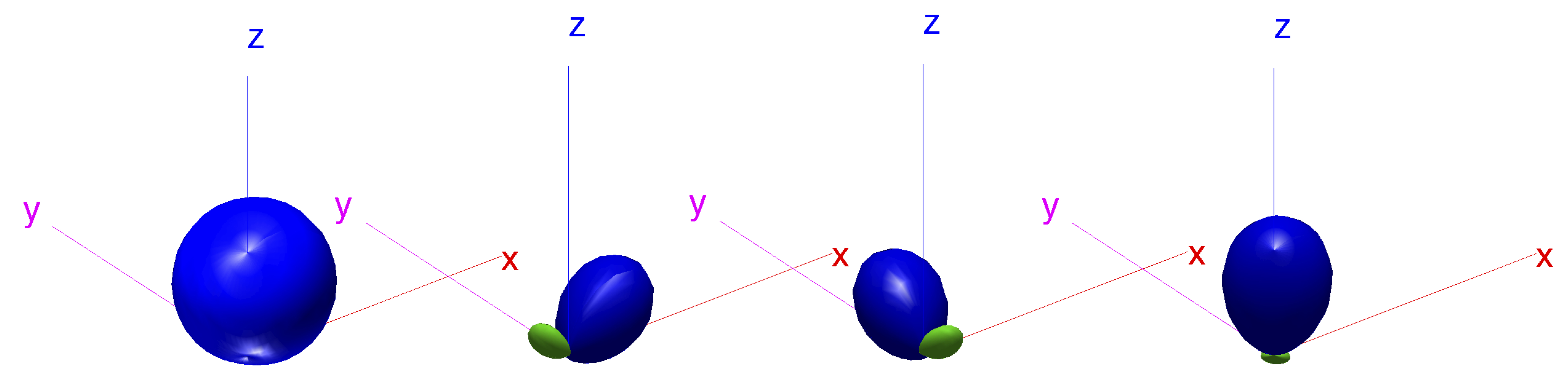
The acoustic velocity components of a plane-wave field spatially-weighted by a beam pattern $\mrm{w}(\Omega)$ can be measured by generating beam patterns $\mrm{w}_\mrm{x}(\Omega),\, \mrm{w}_\mrm{y}(\Omega),\, \mrm{w}_\mathrm{z}(\Omega)$ that are products of the original pattern and the three orthogonal dipoles as in \begin{equation} \label{eq:beam_xyz} \mrm{w}(\Omega)\vb{n}(\Omega) = \left[ {\begin{array}{c} \mrm{w}_\mathrm{x}(\Omega) \\ \mrm{w}_\mathrm{y}(\Omega) \\ \mrm{w}_\mathrm{z}(\Omega) \end{array} } \right] = \left[ {\begin{array}{c} \mrm{w}(\theta, \varphi)\sin\theta \cos\varphi \\ \mrm{w}(\theta, \varphi) \sin\theta \sin\varphi \\ \mrm{w}(\theta, \varphi) \cos\theta \end{array} } \right], \end{equation} where $\Omega = (\theta, \phi)$ is the inclination-azimuth direction of incidence, $\vb{n}(\Omega) = [\sin\theta \cos\phi,\, \sin\theta \sin\phi,\, \cos\theta ]^T$ is the unit vector pointing at $\Omega$. If the beam pattern $\mrm{w}(\Omega)$ is directionally band-limited to order $N-1$, then these velocity patterns are of order $N$, since they are products of the original pattern and the dipole components of $\vb{n}(\Omega)$ which are of order $N=1$.

The problem of computing these patterns is equivalent to the problem of finding their spherical harmonic coefficients, knowing the coefficients of the spatial filter. Let us denote the spherical harmonic transform of the spatial filter as \begin{equation} \label{eq:beam_pat} \vb{w}_{N-1} = \mathcal{SHT}\left[w(\Omega)\right], \end{equation} which returns all $N^2$ spherical harmonic coefficients up to order $N-1$ in a vector $\vb{w}_{N-1}$.The inverse SHT of Eq.\ref{eq:beam_pat} is denoted as \begin{equation} \label{eq:ibeam_pat} w(\Omega) = \mathcal{ISHT}\left[\vb{w}_{N-1}\right]. \end{equation} Similarly the coefficient vectors of the velocity patterns are defined as \begin{equation} \label{eq:beam_pat_xyz} \vb{w}^\mrm{i}_N = \mathcal{SHT}\left[\mrm{w}_\mrm{i}(\Omega)\right], \quad \mrm{with\; i=\{x,y,z\} }, \end{equation} which are of length $(N+1)^2$. The complex SH coefficients of the dipole patterns are given by \begin{align} \label{eq:dipoleSH} [\mathbf{x}_1,\, \mathbf{y}_1,\, \mathbf{z}_1] = \mathcal{SHT}\left[\mrm{x}(\Omega),\, \mrm{y}(\Omega),\, \mrm{z}(\Omega) \right] = \left[ \begin{array}{ccc} 0 & 0 & 0 \\ \sqrt{\frac{2\pi}{3}} & \sqrt{\frac{2\pi}{3}}i & 0\\ 0 & 0 & \sqrt{\frac{4\pi}{3}}\\ -\sqrt{\frac{2\pi}{3}} & \sqrt{\frac{2\pi}{3}}i & 0 \end{array} \right]. \end{align}

Eq.\ref{eq:beam_pat_xyz} is equal to the SHT of the product of the SH series expansion (or the ISHT) of the beam and dipole pattern, as is shown for e.g. the $\mrm{x}$ component \begin{equation} \label{eq:beam_xyz_expand} \vb{w}^\mrm{x}_N = \mathcal{SHT}\left[ \mrm{w}(\Omega)\, \mrm{x}(\Omega) \right] = \mathcal{SHT}\left[\mathcal{ISHT}\left[\vb{w}_{N-1}\right] \cdot \mathcal{ISHT}\left[\vb{x}_1\right] \right]. \end{equation} By manipulating Eq.\ref{eq:beam_xyz_expand}, the result can expressed as a linear combination of the original spatial filter's coefficients $\vb{w}_{N-1}$ as in \begin{equation} \label{eq:beam_xyz_mtx} \vb{w}^\mathrm{i}_N = \vb{A}^\mathrm{i}_N \vb{w}_{N-1},\quad \mathrm{with\; i=\{x,y,z\} }. \end{equation} The matrices $\vb{A}_N^\mathrm{x}, \vb{A}_N^\mathrm{y}, \vb{A}_N^\mathrm{z}$ are $(N+1)^2\times N^2$ sparse deterministic matrices that depend only on dipole coefficients and the order $N$. More specifically, after factoring the result as in Eq.\ref{eq:beam_xyz_mtx}, the matrices $\vb{A}^\mathrm{i}_N$ contain only products of the SH coefficients of the dipoles of Eq.\ref{eq:dipoleSH} and spherical harmonic coupling coefficients $G_{q'q''}^q$ (also termed Gaunt coefficients) as in \begin{align} \label{eq:beam_xyz_terms} {\lfloor\mathbf{A}^\mathrm{x}\rfloor}_{ij} &=& x_1 G_{(j-1)1}^{(i-1)} + x_3 G_{(j-1)3}^{(i-1)} \nonumber\\ {\lfloor\mathbf{A}^\mathrm{y}\rfloor}_{ij} &=& y_1 G_{(j-1)1}^{(i-1)} + y_3 G_{(j-1)3}^{(i-1)} \nonumber\\ {\lfloor\mathbf{A}^\mathrm{z}\rfloor}_{ij} &=& z_2 G_{(j-1)2}^{(i-1)}. \end{align} The Gaunt coefficients $G_{q'q''}^q$ relate the $q'$ and $q''$ coefficient of two spherical functions under multiplication, to the $q$ coefficient of their product, where $q = n(n+1)+m$. The matrices $\vb{A}^\mathrm{i}_N$ can be precomputed analytically for up to some maximum operational order $N$. Then the velocity patterns for any spatial filter up to order $N-1$ can be found directly by Eq.\ref{eq:beam_xyz_mtx}. The Gaunt coefficients can be computed in various ways (Sebilleau1998). In this work they were evaluated through Wigner-3j symbols.

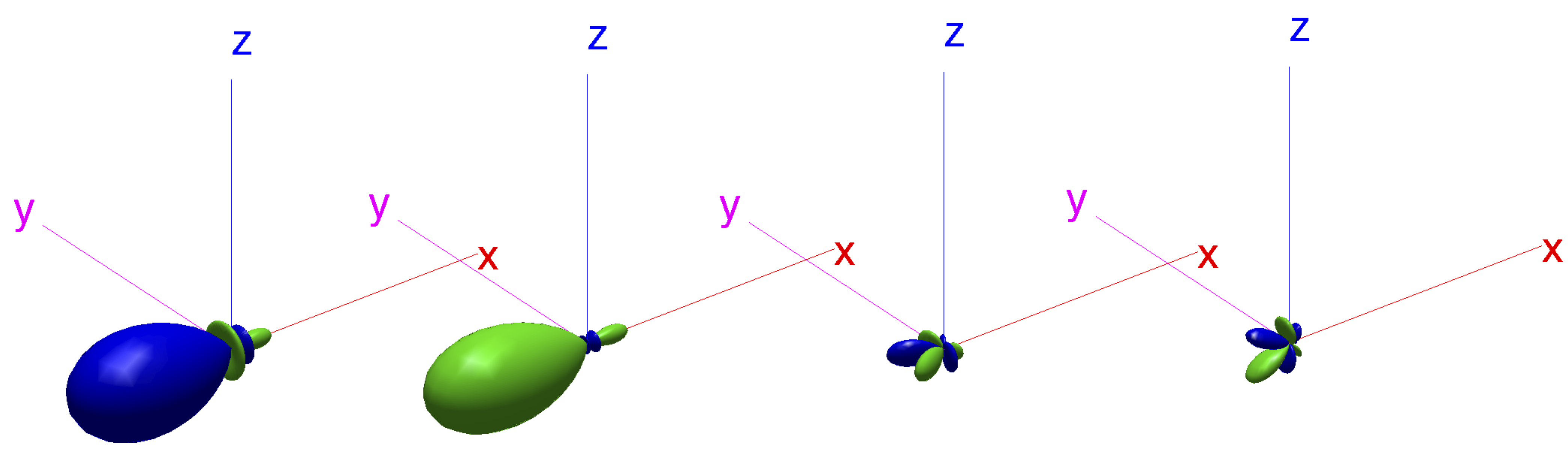
Two examples are plotted below, in which the beam pattern of the spatial filter $\mrm{w}(\Omega)$ is plotted first and then succesively the velocity patterns $\mrm{w}_\mrm{x}(\Omega),\, \mrm{w}_\mrm{y}(\Omega),\, \mrm{w}_\mrm{z}(\Omega)$ follow, from left-to-right.

A Matlab data file (.mat) containing these velocity matrices computed for up to $N-1=20$ order beam patterns can be found here . Note that the derivation assumes fully-orthonormalized complex spherical harmonics, with the Condon-Shortley phase term $(-1)^m$, included either in the definition of the SHs, or in the definition of the associated Legendre functions (as in the case of Matlab's legendre function).

References

D. Sebilleau, On the computation of the integrated products of three spherical harmonics, Journal of Physics A: Mathematical and General, vol. 31, no. 34, p. 7157, 1998.