An Efficient Algorithm for the Restoration of Audio Signals
Corrupted with Low-Frequency Pulses
Paulo A. A. Esquef, Luiz W. P. Biscainho, and Vesa Välimäki
This is a companion web page to a paper that was submitted to the Journal of the Audio Engineering Society in August 2002. Preliminary results of this work have been published in:
P. A.
A. Esquef, L. W. P. Biscainho, V. Välimäki, and M. Karjalainen, "Removal
of
long pulses from audio signals using two-pass split-window filtering," presented
at the AES 112th Convention, Munich, Germany, May 10-13, preprint 5535
1. Abstract
This paper addresses the restoration of audio signals proceeding from old
recordings, and focuses on long-pulse removal. We propose a new two-stage
method to estimate the waveform of each long pulse from the observed noisy
signal. First, an initial estimate for the pulse shape is obtained via a
non-linear filtering scheme called two-pass split-window (TPSW) filtering.
Then, this estimate is further smoothed through a piecewise polynomial fitting.
The degree of smoothness of the estimate can be controlled by adjusting either the
TPSW parameters or the length of the segments to be fitted. The proposed method
has low computational complexity, it is not constrained by the assumption of
shape similarity among pulse waveforms, and can be successfully applied for
removing overlapping pulses.
2. Animated illustration of the variable-length TPSW filtering (section 2 in the paper).
Movie description: the beginning of a segment corrupted with a pulse is the blue curve seen in the first plot. The sliding split-window is seen as red boxes while the output of the first pass is plotted also in red in the curve displayed below. The substituted sequence, which is superposed to the output of the first passs, is plotted in black. Again, the second pass, which is done with a moving-average filter instead of a split-window, is seen as the sliding red box while the corresponding output is drawn in red in the plot below. Finally, the corrupted segment appears in blue for comparison purposes. Place the mouse pointer on the image below to play the movie! Or click here to download the .avi movie (about 5Mb).
3. Algorithm Calibration
The TPSW-based pulse removal system needs an initial calibration. This is an easy task, though. A graphical user interface turns out to be handy for this purpose. From the links below you can download an example of GUI and try yourself!
·
Windows
- Stand alone application for Windows users: SA_GUI.ZIP
- Matlab6 users on Windows: MATLAB6_GUI_WIN.ZIP
- Matlab 6 – R13 on Windows: MATLAB6_R13_GUI_WIN.ZIP
· Linux
- Matlab6 – R12 users on Linux: MATLAB6_GUI_LINUX.ZIP
- Matlab6 – R13 users on Linux: MATLAB6_R13_GUI_LINUX.ZIP
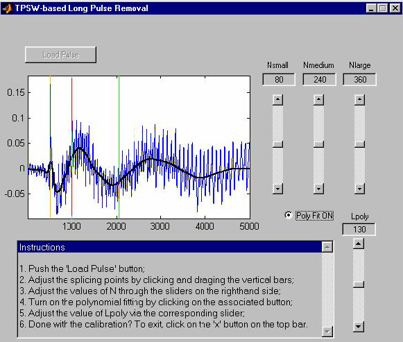
3.1 Basic GUI controls:
Vertical bars (yellow, red, and green): define the splicing
points to assemble the pulse estimate.
Nsmall: controls the smoothness level of the pulse
estimate within the region delimited between the yellow and red bars,
respectively.
Nmedium: controls the smoothness level within the region
defined between the red and green vertical bars.
Nlarge: controls the smoothness level of the estimate in the
region that precedes the yellow bar and in that succeeding the green bar.
Regarding the adustment of Nsmall, Nmedium, and Nlarge, the larger their
values, the smoother the associated estimates become.
Poly Fit ON: Turn ON/OFF the piecewise polynomial fitting.
Lpoly: controls the overall smoothness level of the pulse
estimate. The larger the value of Lpoly, the smoother the pulse estimate
becomes.
4. Performance Assessment
4.1. Description of the Test Signals
1. pop: a 14-second long
exerpt of Finnish pop music with male and female singing;
2. jazz: an 8-second long
excerpt of jazz quartet music with drums, bass, guitar and sax;
3. classic: a
13-second long excerpt of orchestral music with a continuously sustained bass
chord, slowly varying string passage and percussion;
4. ethnic:
an 11-second long excerpt of Brazilian music featuring male singing,
folk fiddle, and prominent percussion beating;
5. drums: an
11-second long solo of jazz drums;
6. bass: a
13-second long of acoustic bass with sparse notes;
7. singing:
a 20-second long excerpt of pop singing a capella.
4.2 Processing Parameters (see tables 1 and 2 in the paper)
4.3. Objective Measures
4.3.1 Segmental Signal-to-Noise Ratio (all values in dB).
For the signal-to-noise ratio (SNR) measure, the higher the value of SNR,
the closer the restored version is to the reference uncorrupted signal.
Theoretically, identical signals (sample-by-sample) would yield an SNR equal to
infinity. From a perceptual point of view, the value of the SNR alone does not
say much about the quality of the evaluated signal. For example, restored
versions with measured values of SNR equal to 120 dB and 300 dB may sound
identical.
|
|
Weak Pulses |
Strong Pulses |
||||
|
|
Corrupted |
TPSW-based |
AR-Separation |
Corrupted |
TPSW-based |
AR-separation |
4.3.2 Logarithm Spectral Distortion (SD). The couplets indicate {average SD in dB, percentage of frames with SD above 2 dB}.
SD measures are widely used to evaluate quality of coded speech. For
instance, speech can be considered transparent (not affect perceptually) to
quantization of the linear prediction coefficients if the quantization scheme
yields average SD below 1 dB and as low as possible percentage of outlier
frames (those with SD > 2 dB). We cannot claim that the same condition holds
when evaluating restored signals, since no listening tests were carried out to
verify such a condition. However, comparing the SD associated with two
different restored versions of a corrupted signal can provide useful insight on
the performance of different algorithms or the appropriate choice of their
processing parameters. Theoretically, the minimum possible value of SD is 0,
which means that the two confronted signals are equal. Objectively, the lower
the value of SD, the closer to the reference the restored version is.
|
|
Weak Pulses |
Strong Pulses |
||||
|
|
Corrupted |
TPSW-based |
AR-separation |
Corrupted |
TPSW-based |
AR-separation |
4.3.3 Perceptual Audio Quality Measure (PAQM)
In the PAQM the reference signal and the signal under test are transformed from the time-domain to a representation that emulates how the signals appear to the inner-ear. Then, a cognitive model interprets the differences between the inner-ear representations of the two signals and provides an overall index of dissimilarity.
Theoretically, the minimum possible value of PAQM is 0, which means that the
reference and evaluated signal are identical from the perceptual point of view.
Note that we assume that the reference signal is the one with highest quality.
Thus, the lower the value of PAQM, the higher the perceptual quality of the
evaluated signal.
|
|
Weak Pulses |
Strong Pulses |
||||
|
|
Corrupted |
TPSW-based |
AR-separation |
Corrupted |
TPSW-based |
AR-separation |
This URL: http://www.acoustics.hut.fi/publications/papers/jaes-LP
Last modified: 11.06.2003
Author: <esquef@acoustics.hut.fi>